 SEARCH
Category Archives: Software
MATLAB R2014b and PLS_Toolbox 7.9
Oct 7, 2014
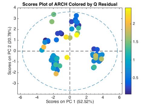
The MathWorks released MATLAB R2014b (version 8.4) last week, and right on its heels we released PLS_Toolbox 7.9. R2014b has a number of improvements that MATLAB and PLS_Toolbox users will appreciate, specifically with graphics. The new MATLAB is more aesthetically pleasing to the eye, easier for the Color Vision Deficiency (CVD) challenged, and smoother due to better anti-aliasing. An example is shown below where the new CVD-friendly Parula color map is used to indicated the Q-residual values of the samples.
But the most significant changes in R2014b are really for people (like us) that program in MATLAB. For instance, TMW didn’t just change the look of the graphics, they actually changed the entire handle graphics system to be object oriented. They also added routines useful in big data applications, and improved their handling of date and time data. When you start the new MATLAB the command window greets you with this:
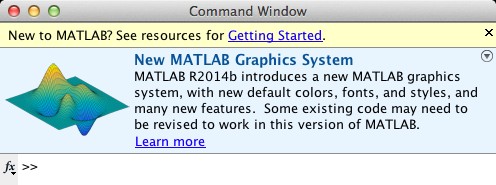
“Some existing code may need to be revised to work in this version of MATLAB.” That is something of an understatement. In fact, R2014b required the update of almost every interface from PLS_Toolbox 7.8. Revising our code to work with R2014b required hundreds of hours. But the good news for our users is that we were ready with PLS_Toolbox 7.9 when R2014b was released AND, as always, we made our code work with previous versions of MATLAB (back to R2008a). This, of course, is the significant difference between a supported commercial product and freeware. Not only do you get new features regularly, but you can rely on it being supported as operating systems and platforms change.
So if you look at the Version 7.9 Release Notes, you won’t see a lot of major changes. Instead, we took the time to assure compatibility with R2014b and made many minor changes to improve usability and stability.
The new MATLAB will allow our command-line and scripting users to do their science more efficiently and present their result more elegantly. These improvements will benefit us as well, and will ultimately translate into continued improvement in PLS_Toolbox and Solo.
BMW
Eigenvector Starts 20th Year
Jan 6, 2014
On New Year’s day 2014 Eigenvector Research, Inc. (EVRI) celebrated its 19th birthday and began its 20th year. The momentum that carried us into 2013 built throughout the year and resulted in our largest year-over-year software sales increase since 2007. Our best three software sales months ever have all been within the last five months. Clearly our partnering with analytical instrument makers and software integrators plus our tools for putting models on-line are striking a responsive chord with users.
The consulting side of our business also continues to be very busy as we assist our clients to develop analytical methods in a wide variety of applications including medical, pharmaceutical, homeland security (threat detection), agriculture, food supplements, energy production and more.
The third leg of our business, chemometrics training, continued unabated as we taught on-site courses for government and industry, courses at conferences and held the 8th edition of our popular Eigenvector University (EigenU). We enter 2014 firing on all cylinders!
Major additions to PLS_Toolbox and Solo in 2013 included the Model Optimizer, Hierarchical Model Builder, a new Artificial Neural Network (ANN) tool, and several new file importers. We will soon release an additional ANN option along with new tools for instrument standardization/calibration transfer. Also on the horizon, a major new release of Solo_Predictor will include an enhanced web interface option and additional instrument control and scripting options.
2014 includes a busy schedule with conferences, talks, conference exhibits and short courses. Below is a listing of where you’ll be able to find us:
- January 21-24, IFPAC, Arlington, VA. BMW to present “Mixed Hierarchical Models for the Process Environment” and “A Multivariate Calibration Model Maintenance Road Map.”
- March 2-6, Pittcon Chicago, IL. NBG and RTR will be at the EVRI exhibition booth.
- April 27-May 2, EigenU 2014, 9th Annual Eigenvector University, Seattle, WA. Join the complete EVRI staff for 6 days of courses and events.
- May 6-9, EuroPACT, Barcelona, Spain. BMW to give plenary address “Model Maintenance: the Unrecognized Cost in PAT and QbD” and a condensed version of our “Chemometrics without Equations” short course.
- June 1-4, CMA4CH, Taormina, Italy. JMS to teach short course and talk TBD.
- June 8-12, CAC-XIV, Richmond, VA. NBG and RB to teach “Advanced Preprocessing for Spectroscopic Applications” and “Alternative Modeling Methods in Chemometrics.”
- August 2-8, IDRC, Chambersburg, PA. NBG to attend, talk TBD.
- September 14-18, ICRM, Nijmegen, The Netherlands. NBG to give keynote “An Overview of Hyperspectral Image Analysis in Chemometrics.”
- September 28-October 3, SciX 2014, Reno, NV. JMS Chemometrics Section Chair, talks and courses TBD.
- November 10-13, EigenU Europe, Hillerød, Denmark. Courses led by BMW and Eigenvector Associate Rasmus Bro.
- November 17-19, EAS 2014, Somerset, NJ. EVRI sponsor of Award for Achievements in Chemometrics. Courses and talks TBD.
We’re especially excited about this year’s Eigenvector University. This ninth edition of EigenU will include all our usual events (poster session, PowerUser Tips & Tricks, workshop dinner) plus five new short courses. Special guest Age Smilde will lead “Chemometrics in Metabolomics” and Rasmus Bro will present “Modeling Fluorescence EEM Data.” The other three new courses are “Calibration Model Maintenance,” “PLS_Toolbox Beyond the Interfaces” and “Getting PLS_Toolbox/Solo Models Online.” We expect EigenU 2014 to be an especially fun and fruitful learning experience.
We look forward to working with you in 2014!
BMW
MATLAB Version Distribution
Jan 24, 2013
One of the challenges of writing software that works with MATLAB is accommodating an array of versions. For better or worse, not everybody updates their MATLAB regularly. So we have to make our PLS_Toolbox and other toolboxes work with a fairly wide distribution of MATLABs.
To give you some idea of what our developers are up against, the plot below shows the distribution of MATLAB versions among our users for each of the last three years. (Click on the plot to get a much larger .pdf version.)

While the most common version in use at any one time tends to be one of the latest two or three releases, it never peaks at more than 20% of our users. And there are LOTS of users with older versions of MATLAB. Note that the plot goes back ten years to 2003! In 2010, we still had 12% of our users with MATLAB versions from 2005 or earlier. It was only after that dropped to less than 5% that we stopped supporting MATLAB 6.5 and 7.0.1 in our new releases. As shown in our release notes, we currently support MATLAB 7.0.4 (from early 2005) through the current MATLAB 8.0 (R2012b). And with our latest minor update (PLS_Toolbox 7.0.3) we’re ready for R2013a, so you’ll be set when it comes out.
But it is a balancing act. We don’t want to force users to upgrade their MATLAB. We understand that an older version of MATLAB works perfectly well for many users. But often we can’t take advantage of newer MATLAB features until we cut old versions loose. As an example, it would be much easier for our developers to use the newer format for coding objects (such as our DataSet Object) that became available in MATLAB 2008a. Until recently, however, 10% of our users were still working with MATLAB 2007b or older.
Our Chief of Technology Development Jeremy M. Shaver notes: Moving users to later versions of MATLAB allows us to utilize better graphical interface tools (making our interfaces easier to use and more powerful), modern hardware architecture (allowing faster processing and better memory management), and other new programming functionality (making the code easier for us to support and for our power-users to understand). Plus, having fewer MATLAB versions to support means we have fewer “special cases” to support in the code. We balance this against our user’s inconvenience and cost in order to achieve the best overall result for our customers!
Well said, Jeremy!
BMW
What’s Unique About Your PLS?
Jan 10, 2013
I got an email from a prospective user of our software the other day that really set me back. Paraphrasing a bit here, it was “Are there any unique features of your PLS algorithm/diagnostics?” The problem with questions like this one is that I never know where to start. But here is what I wrote.
As for “unique features of your pls algorithm,” well, there are numerous ways to calculate a PLS model, but they all pretty much arrive at the same result (which is good). If you’d like to learn more about PLS algorithms and their accuracy, I suggest you have a look at a series of blog posts I did on the subject. See:
Accuracy of PLS Algorithms
Re-orthogonalization of PLS Algorithms
One Last Time on Accuracy of PLS Algorithms
Speed of PLS Algorithms
As to diagnostics, most of the packages use pretty much the same diagnostics, though sometimes they call them by different names. Usually there is a sample distance metric (e.g. T2) and some sort of residual (e.g. Q).
But maybe what you are really looking for is what makes our software unique, rather than our specific PLS algorithm. We have two major packages for chemometrics. The first is our MATLAB-based PLS_Toolbox, the second is our stand-alone product Solo, which is essentially the compiled version of PLS_Toolbox. The two packages provide identical interfaces and share the same model and data formats. The advantage of PLS_Toolbox is that, because it works within the MATLAB environment, it can be run from the command line and functions from it can be incorporated into other analyses. The advantage of Solo is that you don’t have to have MATLAB.
So right off the bat, a unique feature of our software is that there are completely compatible solutions for working with or without MATLAB. And both of these solutions are available on all platforms, including Windows, Mac OSX and Linux. That is unique.
PLS_Toolbox and Solo have the widest available array of analysis methods. This includes PLS and PCA of course, but also PCR, MLR, MCR, PARAFAC, N-PLS, PLS-DA, SIMCA, SVM, KNN, CLS, LWR, MPCA, Cluster Analysis and Batch Maturity. Plus they have a large number of auxiliary tools for Instrument Standardization, Data Transformation, Dynamic Modeling, Sample Selection, Trend Analysis, Correlation Spectroscopy and Design of Experiments. And numerous tools for variable selection including Genetic Algortihm, iPLS and Stepwise MLR. Plus diagnostic methods such as VIP and Selectivity Ratio. The collection of all of these analysis methods and auxiliary functions with one interface is unique.
PLS_Toolbox and Solo can be extended for use with Multivariate Images with MIA_Toolbox and Solo+MIA. The ability to apply such a wide array of multivariate analysis techniques to images is unique. There is also an add-on for the patented Extended Multiplicative Scatter Correction, EMSC_Toolbox. If not completely unique, this method for preprocessing data from highly scattering samples is not widely available.
For on-line application there is our Solo_Predictor and Model_Exporter. Solo_Predictor can be used with any model generated by PLS_Toolbox/Solo and can communicate via TCP/IP sockets, ActiveX, .NET, timed action or wait-for-file. Model_Exporter translates PLS_Toolbox/Solo models into mathematical formulas that can be compiled into other languages. Model_Exporter’s XML output can be parsed for execution in .NET (C#). Additional output formats include MATLAB .m file (compatible with older versions of MATLAB and OCTAVE, plus LabView, Symbion and Tcl). This wide array of on-line options is unique.
Beyond that, PLS_Toolbox and Solo are also extremely flexible tools and include the widest array of data preprocessing methods with user-specified ordering, ability to add user-specified method, and customizable favorites settings.
And finally, price. PLS_Toolbox is only $1395 for industrial users, $395 for academic. Solo is $2195/$695. The price/performance ratio of these products is most certainly unique.
If you have any questions about the specific functionality of our software, please write me.
BMW
Find Jeremy Shaver at EAS Next Week
Nov 8, 2012
Eigenvector’s Chief of Technology Development Dr. Jeremy Shaver is getting ready to head off to the Eastern Analytical Symposium (EAS). He’ll be busy on Sunday and Monday assisting Eigenvector Associate Dr. Don Dahlberg with Chemometrics without Equations (CWE). As I wrote previously, this year the popular CWE is being extended by a day to cover advanced data preprocessing. Jeremy will be demonstrating the methods using the recently released PLS_Toolbox/Solo 7.0. If you’d like to attend, there is still time to register through the conference web site!
Jeremy will also represent EVRI at the session honoring Professor Dr. Lutgarde Buydens of Radboud University Nijmegen for Outstanding Achievements in Chemometrics. The award is, once again, sponsored by Eigenvector Research. The award session, chaired by University of Barcelona’s Dr. Anna de Juan, will start Monday morning at 9:00am.
You might also find Dr. Shaver at the Cobalt Light Systems Ltd booth. Cobalt, one of EVRI’s Technology Partners, develops tools for non-invasive analysis. Their TRS100 pharmaceutical analysis instrument utilizes our Solo software for chemometric modeling. Jeremy will be there to advise users on how to best calibrate the system for their particular needs.
Of course, if you can catch him, Jeremy would be happy to talk to anyone interested in EVRI’s software offerings! He’s the Eigenvectorian most intimately familiar with our products and their features and capabilities. Drop Dr. Shaver an email if you’d like to meet him at EAS.
Have a good week!
BMW
New Releases: PLS_Toolbox/Solo/Solo+MIA 7.0, MIA_Toolbox 2.8
Oct 30, 2012
New versions of our MATLAB-based PLS_Toolbox and MIA_Toolbox were released earlier this month, along with updates to our stand-alone packages Solo and Solo+MIA. PLS_Toolbox and its derivatives, Solo and Solo+MIA, are now in version 7.0, while MIA_Toolbox is in version 2.8. As can be seen in the release notes, the list of enhancements and additions is long (as usual!).
Many of the new features are demonstrated in the new EigenGuide video, “What’s New in Version 7.0.” The video illustrates the use of:
- additional information in the Analysis interface, such as error of cross-validation
- interfaces for splitting data sets into calibration and validation sets
- tools for visualizing the difference between samples for both their Q residuals and T2 contributions
- simplified control of plot attributes
- readily available class statistics
- automated peak finding
- tools for finding specific samples and variables based on logical operators
Of particular note in this release is the expansion of the Batch Process Modeling tools. The Batch Processor tool readies data sets for modeling by Summary PCA, Batch Maturity, MPCA, and several PARAFAC variants. It then pushes the data sets into the Analysis tool where the models are developed. To see the Batch Processor and Analysis in action, watch the video. The combination of the Batch Processor and methods supported in the Analysis interface allows modelers to follow most of the pathways outlined in my TRICAP 2012 talk, “Getting to Multiway: A Roadmap for Batch Process Data.”
This release reaffirms EVRI’s commitment to continuous software improvement – it completes our fifth year of semiannual major releases. The best chemometrics software just keeps getting better!
BMW
Chemometrics Software for Classroom Use
Sep 17, 2012
Autumn is nearly here and with it comes the first semester of the school year. This morning I was greeted by a sign of fall: a slew of student account creation notifications, drifting into my email inbox like falling leaves.
At EVRI, we work with professors to make our software freely available to students enrolled in chemometrics courses. Students can get free 6-month demo licenses of our MATLAB-based PLS_Toolbox and MIA_Toolbox, or stand-alone Solo or Solo+MIA.
I traded emails this morning with Professor Anna de Juan of the Universitat de Barcelona. This will be the third year we’ve worked with Prof. de Juan on her chemometrics class. She wrote, “we had a very good experience the two semesters using PLS_Toolbox in the classroom. The students were happy and only a pair of them had problems of installation at home. It really made it easy that they could play with proposed data sets out of the classroom, at their own pace and exploring many possibilities.” de Juan noted her students typically use Solo at home because they generally don’t have personal copies of MATLAB.
Another advantage of Solo is that it is available for multiple platforms, including Windows, Linux and Mac OS X. I see lots of Apple laptops on college campuses. A search of the web reveals estimates ranging from 30-70% of college students using Macs. We see a substantial number of student downloads of our Solo for Mac, and expect that number to grow.
Interested in teaching Chemometrics? Drop me a line and we’ll be happy to work with you to provide software for your students.
BMW
New Releases: PLS_Toolbox and Solo 6.7, MIA_Toolbox 2.7
Mar 20, 2012
Updates to our flagship PLS_Toolbox and Solo were released last week; they are now in version 6.7. This is in keeping with our policy, (began in 2008), to release significant upgrades twice yearly. Our Multivariate Image Analysis (MIA) tools were also updated with the release of Solo+MIA 6.7 and MIA_Toolbox 2.7.
As the Version 6.7 Release Notes show, the number of additions, improvements and refinements is (once again!) rather long. My favorite new features are the Drag and Drop import of data files, Confusion Table including cross-validation results for classification problems, and Custom Color-By values for plotting.
PLS_Toolbox/Solo can import a wide variety of file types, and the list continues to grow. Drag and Drop importing allows users to drag their data files directly to the Browse or Analysis windows. They will be loaded and ready for analysis. For instance, users can drag a number of .spc files directly into Analysis. Forget some files or have additional files in a different directory? Just drag them in and they will be augmented onto the existing data.
The Confusion Table feature creates several tables summarizing the classification performance of models. This includes a “confusion matrix” giving fractions of true positive, false positive, true negative, and false negative samples and a confusion table which gives number of samples the actual and predicted classes. Tables are calculated for both the full fitted model and for the cross-validation results. The tables can be easily copy and pasted, saved to file, or can be included in the Report Writer output as html, MS Word or PowerPoint files.
With Custom Color-By users can color points in scores and loadings plots using any currently loaded data or with new data loaded from the workspace. For instance, samples in a PLS LV-2 versus LV-1 scores plot can be colored by the scores on another LV, their actual or predicted y values, leverage, Q residual, specific X-variable, additional Y-variable, or any custom variable from the work space. The allows deeper investigation into the cause of specific variations seen in the data.
Want to find out more about our latest releases? Create an account in our system and you’ll be able to download free 30-day demos. Want prices? No need to sit through a webinar! Just check our price list page, which includes all our products. Just click Academic or Industrial.
As always, users with current Maintenance Agreements can download the new versions from their accounts.
Questions? I’d be happy to answer them or refer you to our development team. Just email me!
BMW
PLS_Toolbox in Research and Publications
Dec 6, 2011
Our Chief of Technology Development Jeremy M. Shaver received a very nice letter this morning from Balázs Vajna, who is a Ph.D. student at Budapest University of Technology and Economics. As you’ll see from the references below, he is a very productive young man! Here is his letter to Jeremy, highlighting how he used PLS_Toolbox in his work:
Dear Jeremy,
I would like to thank you for all your help with the Eigenvector products. With your help, I was able to successfully carry out detailed investigations using chemical imaging and chemometric evaluation in such a way that I could publish these results in relevant international journals. I would like to draw your attention to the following publications where (only) PLS_Toolbox was used for chemometric evaluation:
- B. Vajna, I. Farkas, A. Farkas, H. Pataki, Zs. Nagy, J. Madarász, Gy. Marosi, “Characterization of drug-cyclodextrin formulations using Raman mapping and multivariate curve resolution,” Journal of Pharmaceutical and Biomedical Analysis, 56, 38-44, 2011.
- B. Vajna, H. Pataki, Zs. Nagy, I. Farkas, Gy. Marosi, “Characterization of melt extruded and conventional Isoptin formulations using Raman chemical imaging and chemometrics,” International Journal of Pharmaceutics, 419, 107-113, 2011.
These may be considered as showcases of using PLS_Toolbox in Raman chemical imaging, and – which is maybe even more interesting in the light of your collaboration with Horiba Jobin Yvon – the joint use of PLS_Toolbox and LabSpec. The following studies have also been published where MCR-ALS and SMMA (Purity) were carried out with PLS_Toolbox and were tested along with other curve resolution techniques.
- B. Vajna, G. Patyi, Zs. Nagy, A. Farkas, Gy. Marosi, “Comparison of chemometric methods in the analysis of pharmaceuticals with hyperspectral Raman imaging,” Journal of Raman Spectroscopy, 42(11), 1977-1986, 2011.
- B. Vajna, A. Farkas, H. Pataki, Zs. Zsigmond, T. Igricz, Gy. Marosi, “Testing the performance of pure spectrum resolution from Raman hyperspectral images of differently manufactured pharmaceutical tablets,” Analytica Chimica Acta, in press.
- B. Vajna, B. Bodzay, A. Toldy, I. Farkas, T. Igricz, G. Marosi, “Analysis of car shredder polymer waste with Raman mapping and chemometrics,” Express Polymer Letters, 6(2), 107-119, 2012.
I just wanted to let you know that these publications exist, all using PLS_Toolbox in the evaluaton of Raman images, and that I am very grateful for your help throughout. I hope you will find them interesting.
Best regards,
Balázs
—
Balázs Vajna
PhD student
Department of Organic Chemistry and Technology
Budapest University of Technology and Economics
8 Budafoki str., H-1111 Budapest, Hungary
Thanks, Balázs, your letter just made our day! We’re glad you found our tools useful!
BMW
Missing Data (part three)
Nov 21, 2011
In the first and second installments of this series, we considered aspects of using an existing PCA model to replace missing variables. In this third part, we’ll move on to using PLS models.
Although it was shown previously that PCA can be used to perfectly impute missing values in rank deficient, noise free data, it’s not hard to guess that PCA might be suboptimal with regards to imputing missing elements in real, noisy data. The goal of PCA, after all, is to estimate the data subspace, not predict particular elements. Prediction is typically the goal of regression methods, such as Partial Least Squares. In fact, regression models can be used to construct estimates of any and all variables in a data set based on the remaining variables. In our 1989 AIChE paper we proposed comparing those estimates to actual values for the purpose of fault detection. Later this became known as regression adjusted variables, as in Hawkins, 1991.
There is a little known function in PLS_Toolbox, (since the first version in 1989 or 90), plsrsgn, that can be used to develop collections of PLS models, where each variable in a data set is predicted by the remaining variables. The regression vectors are mapped into a matrix that generates the residuals between the actual and predicted values in much the same way as the I–PP‘ matrix from PCA.

We can compare the results of using these collections of PLS models to using the PCA done previously. Here we created the coeff matrix using (a conservative) 3 LVs in each of the PLS submodels. Each sub model could of course be optimized individually, but for illustration purposes this will be adequate. The reconstruction error of the PLS models is compared with PCA in the figure shown at left, where the error for the collection of PLS models is shown in red, superimposed over the reconstruction via the PCA model error, in blue. The PLS models’ error is lower for each variable, in some cases, substantially, e.g. variables 3-5.
![]()
The second figure, at left, shows the estimate of variable 5 for both the PLS (green) and PCA (red) methods compared to the measured values (blue). It is clear that the PLS model tracks the actual value much better.
Because the estimation error is smaller, collections of PLS models can be much more sensitive to process faults than PCA models, particularly individual sensor faults.
It is also possible to replace missing variables based on these collections of PLS models in (nearly) exactly the same manner as in PCA. The difference is that, unlike in PCA, the matrix which generates the residuals is not symmetric, so the R12 term (see part one) does not equal R21‘. The solution is to calculate b using their average, thus
b = 0.5(R12 + R21‘)R11-1
Curiously, unlike the PCA case, the residuals on the replaced variables will not be zero except in the unlikely case that R12 = R21‘.
In the case of an existing single PLS model, it is of course possible to use this methodology to estimate the values of missing variables based on the PLS loadings. (Or, if you insist, on the PLS weights. Given that residuals based on weights are larger than residuals based on loadings, I’d expect better luck reconstructing from the loadings but I offer that here without proof.)
In the next installment of this series, we will consider the more challenging problem of building models on incomplete data records.
BMW
B.M. Wise, N.L. Ricker, and D.J. Veltkamp, “Upset and Sensor Failure Detection in Multivariate Pocesses,” AIChE Annual Meeting, 1989.
D.M. Hawkins, “Multivariate Quality Control Based on Regression Adjusted Variables,” Technometrics, Vol. 33, No. 1, 1991.
Missing Data (part two)
Nov 11, 2011
In Missing Data (part one) I outlined an approach for in-filling missing data when applying an existing Principal Components Analysis (PCA) model. Let us now consider when this approach might be expected to fail. Recall that missing data estimation results in a least-squares problem with solution:
xb = –xgR21R11-1
In our short courses, I advise students to be wary any time a matrix inverse is used, and this case is no exception. Inverses are defined only for matrices of full rank, and may be unstable for nearly rank-deficient matrices. So under what conditions might we expect R11 to be rank deficient? Recall that R11 is the part of I–PP‘ that applies to the variables which we want to replace. Problems arise when the variables to be replaced form a group that are perfectly correlated with each other but not with any of the remaining variables. When this happens the variables will either be 1: included as a group in the PCA model (if enough PCs are retained) or 2: excluded as a group (too few PCs retained). In case 1, R11 is rank deficient and the inverse isn’t defined. In case 2, R11 is just I, but the loadings of the correlated group are zero, so the R12 part of the solution is 0. In either case, it makes sense that a solution isn’t possible–what information would it be based on?
With real data, of course, it is highly unlikely that R11 will be rank deficient to within numerical precision (or that R12 will be zero). But it certainly may happen that R11 is near rank deficient, in which case the estimates of the missing variables will not be very good. Fortunately, in most systems the measured variables are somewhat correlated with each other and the method can be employed.

In their 1995 paper, Nomikos and MacGregor estimated the value of missing variables using a truncated Classical Least Squares (CLS) formulation. The PCA loadings are fit to the available data, leaving out the missing portions, to estimate scores which are then used to estimate missing values. This reduces to:
xb = xg(PgPg‘)-1PgPb‘
where Pb and Pg refer to the part of the PCA model loadings for the missing (bad) and available (good) data, respectively. In 1996 Nelson, Taylor and MacGregor noted that this method was equivalent to the method in our 1991 paper but offered no proof. The proof can be found in “Refitting PCA, MPCA and PARAFAC Models to Incomplete Data Records” from FACSS, 2007.

So how does this work in practice? The topmost figure shows the estimation error for each of the 20 variables in the melter data based on a 4 PC models with mean-centering. The model was estimated with every other sample and tested on the other samples. The estimation error is shown in units of Relative Standard Deviation (RSD) to the raw data. Thus, the variables with error near 1.0 aren’t being predicted any better than just using the mean value, while the variables with error below 0.2 are tracking quite well. An example is shown in the middle figure, which shows temperature sensor number 8 actual (blue line) and predicted (red x) for the test set as a function sample number (time).

The reason for the large differences in ability to replace variables in this data set is, of course, directly related to how independent the variables are. A graphic illustration of this can be produced with the PLS_Toolbox corrmap function, which produced the third figure. The correlation matrix for the temperatures is colored red where there is high positive correlation, blue for negative correlation, and white for no correlation. It can be seen that variables with low estimation error (e.g. 7, 8, 17, 18) are strongly correlated with other variables, whereas variables with high estimation error (e.g. 2, 12) are not correlated strongly with any other variables.
To summarize, we’ve shown that missing variables can be imputed based on an existing PCA model and the available measurements. This success of this approach depends upon the degree to which the missing variables are correlated with available variables, as might be expected. In the next installment of this Missing Data series, we’ll explore using regression models, particularly Partial Least Squares (PLS) to replace missing data.
BMW
P. Nomikos and J.F. MacGregor, “Multivariate SPC Charts for Monitoring Batch Processes,” Technometrics, 37(1), pps. 41-58, 1995.
P.R.C. Nelson, P.A. Taylor and J.F. MacGregor, “Missing data method in PCA and PLS: Score calculations with incomplete observations,” Chemometrics & Intell. Lab. Sys., 35(1), pps. 45-65, 1996.
B.M. Wise, “Re-fitting PCA, MPCA and PARAFAC Models to Incomplete Data Records,” FACSS, Memphis, TN, October, 2007.
Missing Data (part one)
Nov 5, 2011
Over the next few weeks I’m going to be discussing some aspects of missing data. This is an important aspect of chemometrics as many applications suffer from this problem. Missing data is especially common in process applications where there are many independent sensors.
I got interested in missing data while in graduate school in the late 1980s. I worked a lot with a prototype glass melter for the solidification of nuclear fuel reprocessing waste. The primary measurements were temperatures provided by thermocouple sensors. The very high temperatures in this system, nearing 1200C (~2200F), caused the thermocouples to fail frequently. Thus it was common for the data record to be incomplete.
Missing data is also common in batch process monitoring. There are several approaches for building models on complete, finished batches. However, it is most useful to know if batches are going wrong BEFORE they are complete. Thus, it is desirable to be able to apply the model to an incomplete data record.
Missing data problems can be divided into two classes: 1)those involving missing data when applying an existing model to new data records, and 2) those involving building a model on an incomplete data record. Of these, the first problem is by far the easiest to deal with, so we will start with it. It will, however, illustrate some approaches which can be modified for use in the second case. These approaches can also be used for other purposes as well, such as cross-validation of Principal Component Analysis (PCA) models.
Consider now the case where you have a process that periodically produces a new data vector xi (1 x n). With it you have a validated PCA model, with loadings Pk (n x k). The residual sum-of-squares or Q statistic, can be calculated for the ith sample as Q = xiRxi‘ where R = I–PkPk‘. For the sake of convenience, imagine that the first p variables in this model are no longer available, but the remaining n–p variables are as usual. Thus, x can be partitioned into a group of bad variables xb and a group of good variables xg, x = [xb xg]. The calculation of Q can then be broken down into parts which do and do not involve missing variables:
Q = xbR11xb‘ + xgR21xb‘ + xbR12xg‘ + xgR22xg‘
where R11 is the upper left (p x p) part of R, R12 = R21‘ is the lower left (n–p x p) section, and R22 is the lower right (n–p x n–p) section.
It is possible to solve for the values of the bad variables xb that minimize Q, as shown in our 1991 paper referenced below. The (incredibly simple) solution is
xb = –xgR21R11-1
Unsurprisingly, the residuals on the replaced variables on the full model will be zero.
This method is the basis of the PLS_Toolbox function replace, which maps the solution above into a matrix so variables in arbitrary positions can be replaced.

It is easy to demonstrate that this method works perfectly in the rank deficient, no noise case. In MATLAB, you can create a rank 5 data set with 20 variables, then use the Singular Value Decomposition (SVD) to get a set of PCA loadings P, and from that, the R matrix.
>> c = randn(100,5);
>> p = randn(20,5);
>> x = c*p’;
>> [u,s,v] = svd(x);
>> P = v(:,1:5);
>> R = eye(20)-P*P’;
Now let’s say the sensor associated with variable 5 has failed. We can use the replace function to generate a matrix Rm which replaces it based on the values of the other variables.
>> Rm = replace(R,5,’matrix’);
>> imagesc(sign(Rm)), colormap(rwb)
Rm has the somewhat curious structure show in the figure above. The white area is zeros, the diagonal is ones, and R21R11-1 for the appropriately rearranged R is mapped into the vertical section.

We can try Rm out on a new data set that spans the same space as the previous one, and plot up the results as follows:
>> newx = randn(100,5)*p’;
>> var5 = newx(:,5);
>> newx(:,5) = 0;
>> newx_r = newx*Rm;
>> figure(2)
>> plot(var5,newx_r(:,5),’+b’), dp
The (not very interesting) figure at left shows that the replaced value of variable 5 agrees with the original value. This can be done for multiple variables.
In the second installment of this Missing Data series I’ll give some examples of how this works in practice, discuss limitations, and show some alternate ways of estimating missing values. In the third installment we’ll get to the much more challenging issue of building models on incomplete data sets.
BMW
B.M. Wise and N.L. Ricker, “Recent advances in Multivariate Statistical Process Control, Improving Robustness and Sensitivity,” IFAC Symposium n Advanced Control of Chemical Processes, pps. 125-130, Toulouse, France, October 1991.
PLS_Toolbox/Solo Advanced Features in NJ
Nov 2, 2011
Eigenvector Vice-president Neal B. Gallagher and Chief of Technology Development Jeremy M. Shaver will present Using the Advanced Features in PLS_Toolbox/Solo 6.5 in New Brunswick, NJ on December 8-9, 2011. The course will be held at the Hyatt Regency.
With PLS_Toolbox and Solo Version 6.5 released last month, this is an opportune time to attend this course. Participants will learn how to take advantage of many of the recently added tools. It will also be a great time to ask “how to” type questions. Nobody knows our software more intimately than Jeremy, as he is responsible for its overall development. He’s constantly surprising the rest of us EigenGuys by showing us easier ways to accomplish our modeling tasks using features we didn’t know existed! Neal will be on hand to guide users through many of the methods, particularly the advanced preprocessing features. Neal has extensive experience in this area due to his work with remote sensing applications.
The course includes an optional second half day which covers our tools for Multivariate Image Analysis and Design of Experiments. There will also be time for one-on-one consulting with the software. Attendees are encouraged to bring their own data for this! Often all the methods and tools make a lot more sense when applied to data with which you are familiar.
If you have any questions about this course or our other course offerings, such as EigenU, please write to me.
BMW
Multi-platform Chemometrics Software
Oct 14, 2011
When I go to conferences I often look around to see what sort of computers people are using. In the past year or so I’ve noticed a significant uptick in the number of Macs. At SSC-12, SIMS-XVIII and FACSS/SCIX-2011 Macs accounted for about half of the laptops that I saw in use in the technical sessions and the trade shows.
So, who is making chemometrics software for anything besides Windows? Umetrics isn’t. SIMCA is Windows only. CAMO isn’t. Unscrambler® X is Windows only. Infometrix isn’t. Pirouette® is Windows only. The answer, of course, is Eigenvector Research. Because MATLAB® is available on all platforms, EVRI’s flagship PLS_Toolbox, plus our MIA_Toolbox and EMSC_Toolbox work on Mac OS X, Linux and Windows too. And that includes the 64-bit versions!
Don’t have MATLAB? Not a problem. Our stand-alone packages Solo and Solo+MIA also run on all platforms, including the 64-bit versions. Even our on-line prediction engine, Solo_Predictor, runs on all platforms.
So, besides the fact that PLS_Toolbox and Solo support a wider array of chemometric methods and preprocessing options, and the fact that their point-and-click interfaces are highly intuitive, you can add the fact that they run on more than just Windows. And as if that weren’t enough, they also cost less.
So if you are looking for great chemometrics software that runs in a multi-platform environment, EVRI has solutions for you!
BMW
Unscrambler® is a registered trademark of CAMO, Inc.
Pirouette® is a registered trademark of Infometrix, Inc.
MATLAB® is a registered trademark of The MathWorks, Inc.
Off to FACSS, PLS_Toolbox/Solo 6.5
Sep 30, 2011
The Federation of Analytical Chemistry and Spectroscopy Societies (FACSS) annual meeting starts this Sunday, October 2, in Reno, NV. The EVRI crew headed there includes Neal B. Gallagher (NBG), Jeremy M. Shaver (JMS), Randy Bishop (RB), and myself (BMW). We expect to be busy! We have a number of papers to give, listed below.
- Visualizing Results: Data Fusion and Analysis for Hyperspectral Images, by JMS, Eunah Lee and Karen Gall, Monday, 2:30pm
- Detection of Adulterants in Raw Materials Utilizing Hyperspectral Imaging with Target and Anomaly Detection Algorithms, by Lam K. Nguyen and Eli Margilith of Opotek, NBG and JMS, Tuesday, 4:50pm
- Multivariate Modeling of Batch Processes Using Summary Variables, by BMW and NBG, Wednesday, 10:30am
- A Comparison of Detection Strategies for Solids and Organic Liquids on Surfaces Using Long Wave Infrared Hyperspectral Imaging, by NBG, and Thomas A. Blake and James F. Kelly of PNNL, Wednesday, 1:50pm
We’ll also be in the exhibition hall in Booth #29 demoing the soon-to-be released PLS_Toolbox/Solo version 6.5. As usual, our programing team has been very productive, and the list of new features in 6.5 is very long. We’re especially excited about the new Design of Experiments tools and the streamlining and unification of all our Classification Methods. Stop by and have a look, we’d sure like to show you what’s new.
See you there!
BMW
Solo 6.3 Released
Jun 30, 2011
Version 6.3 of our Solo software products were released this week. This includes the core Solo package, Solo+MIA and Solo+Model_Exporter. This release includes significant improvements to underlying libraries to make Solo faster, more memory friendly, make better use of multi-core processors, and have a more modern look and feel. Details can be found on the Solo 6.3 Release Notes page.
Solo+Model_Exporter 6.3 incorporates the latest Model_Exporter 2.5 which adds support for more preprocessing methods, improved memory support, and includes the freely-distributable .NET prediction engine (Model_Exporter Interpreter) for 3rd party integration. For detailed information, please see the Model_Exporter 2.5 Release Notes.
I asked our Chief of Technology Development, Jeremy M. Shaver, a few questions about the release.
BMW: Can Solo users expect to see performance gains?
JMS: If you use a system with multiple cores, or regularly work with data that is graphically-intensive or generally large, you should expect to see performance gains. If you are using Windows Vista or Windows 7, you can expect to see interfaces which are more consistent with the operating system’s overall look and feel.
BMW: What does this mean for people trying to get models on-line?
JMS: The changes to Solo+Model_Exporter include more support for models with complex preprocessing and improved memory handling. It also includes the new freely distributable .NET object Model_Exporter Interpreter. This object can be integrated into third party .NET applications to easily get exported Solo models on-line. There is no royalty payments associated with either exporting a model or distributing the Interpreter.
BMW: Any impact for hand-held devices?
JMS: The Model_Exporter improvements in memory management also make exported Solo models more hand-held device friendly. In addition, the Model_Exporter Interpreter also makes integrating these models into existing applications much easier.
For more information about what’s been added to Solo (and PLS_Toolbox) in recent releases please see the PLS_Toolbox/Solo Release Notes.
Solo users with current maintenance contracts can upgrade now. Free demos are also available to those with accounts in our system. Don’t have an account? Start by creating one.
BMW
iPods Ordered!
Apr 25, 2011
EigenU 2011 is now less than 3 weeks away: it starts on Sunday, May 15. Once again we’ll have the “PLS_Toolbox/Solo User Poster Session” where users can showcase their own chemometric achievements. This Tuesday evening event is open to all EigenU participants, as well as anyone with a poster which demonstrates how PLS_Toolbox or Solo was used in their work. Presenters of the two best posters will receive Apple iPod nanos for their effort. I ordered them today, (16G, one blue, one orange), engraved with EigenU 2011 Best Poster.
Tuesday evening will also include a short User Group meeting. We’ll give a short presentation highlighting the key features in our latest software releases and discuss directions for future development. Here is your chance to give us your wish list!
The poster session will feature complimentary hors d’oeuvres and beverages. This is a great time to mingle with colleagues and the Eigenvectorians and discuss the many ways in which chemometric methods are used.
See you in May!
BMW
“This software is awesome!”
Apr 7, 2011
That’s what Eigenvector’s Vice-President, Neal B. Gallagher, wrote to our developers, Jeremy, Scott and Donal, this morning about the latest version of PLS_Toolbox. So, OK, he may be a little biased. But it underscores a point, which is that all of us at EVRI who do consulting (including Neal, Jeremy, Bob, Randy, Willem and myself) use our software constantly to do the same type of tasks our users must accomplish. We write it for our own use as well as theirs. (Scott pointed out that this is known as “eating your own dog food.”)
Neal went on to say, “Every time I turn around, this package and set of solutions just keeps getting better and more extensive. I am truly convinced that this is the most useful package of its kind on the market. This is due to your intelligence, foresight, and attention to detail. It is also due to your open mindedness and willingness to listen to your users.”
Thanks, Neal. I think you made EVRIbody’s day!
BMW
Improved Model_Exporter Coming Soon
Mar 29, 2011
EVRI’s Model_Exporter allows users of PLS_Toolbox and Solo to export their Principal Component Analysis (PCA), Partial Least Squares (PLS) Regression and other models in a variety of formats suitable for use in both MATLAB and other environments (e.g. LabSpec, GNU Octave, Symbion, LabVIEW, Java, C++/C#). A new, improved version of Model_Exporter will be released in the coming weeks. The new version will allow models to be more easily applied on platforms with less computer power, such as on hand-held devices.
The new Model_Exporter will include a number of improvements including a much less memory-intensive encoding of Savitzky-Golay derivatives and smoothing and similar improvements in handling of excluded variables. The new version will also support additional preprocessing methods which were released in versions 6.0 and 6.2 of PLS_Toolbox and Solo.
The other big news is that we will also be bundling with Model_Exporter a freely-distributable .NET class to do predictions from exported models. As-is, this class can be integrated into any .NET application (C++/C#/VB) from Microsoft Visual Studio 2005 or later. It can be used and redistributed without any per-use charge (exactly as the exported models are licensed) and we’d be happy to work with you on integrating this class into your end application. If you have interest in this approach, just let our Chief of Technology Development, Jeremy Shaver, or me know.
BMW
PLS_Toolbox or Solo?
Mar 28, 2011
Customers who are new to chemometrics often ask us if they should purchase our MATLAB-based PLS_Toolbox or stand-alone Solo. I’ll get to some suggestions in a bit, but first it is useful to clarify the relationship between the two packages: Solo is the compiled version of the PLS_Toolbox tools which are accessible from the interfaces. Similarly, Solo+MIA is the compiled version of PLS_Toolbox and MIA_Toolbox. The packages share the same code-base, which is great for the overall stability of the software as they operate identically. They are also completely compatible, so PLS_Toolbox and Solo users can share data, models, preprocessing, and results. Models from each are equally easily applied on-line using Solo_Predictor.
The majority of the functionality of PLS_Toolbox is accessible in Solo, particularly the most commonly used tools. Every method that you access through the main Graphical User Interfaces (GUIs) of PLS_Toolbox is identical in Solo. But with Solo you don’t get the MATLAB command line, so there are some command-line only functions that are not accessible. The number of these, however, is decreasing all the time as we make more PLS_Toolbox functionality accessible through the GUIs. And of course all the GUIs in PLS_Toolbox + MIA_Toolbox are accessible in Solo+MIA.
So what to buy? Well, do you already have access to MATLAB? Over one million people do, and it is available in many universities and large corporations. If you have access to MATLAB, then buy PLS_Toolbox (and MIA_Toolbox). It costs less than Solo (and Solo+MIA), includes all the functionality of Solo and then some, can be accessed via command line and called in MATLAB scripts and functions.
And if you don’t already have MATLAB? If you only need to use the mainstream modeling and analysis functions, then Solo (and Solo+MIA) will save you some money over purchasing MATLAB and PLS_Toolbox (and MIA_Toolbox). I’d only purchase MATLAB if I needed to write custom scripts and functions that call PLS_Toolbox functions. Honestly, the vast majority of our users can do what they need to do using the GUIs. The stuff you can’t get to from the GUIs is pretty much just for power users.
That said, the big plus about buying MATLAB plus PLS_Toolbox is that you get MATLAB, which is a tremendously useful tool in its own right. Once you start using it, you’ll find lots of things to do with it besides just chemometrics.
Hope that helps!
BMW