“The age-old concept of data modeling with spectroscopy has been revitalized through the integration of Machine Learning and AI initiatives. The pharmaceutical industry, in particular, is embracing data science, exploring the potential of deep learning and AI tools in spectroscopy applications. The emergence of open-source tools adds transparency to the ‘black box’ of these advanced technologies, sparking discussions around regulatory concerns.”
I’ve been doing data modeling and spectroscopy for 35+ years now and I’ve never felt particularly un-vital (vital–adjective; full of energy, lively). However, there is certainly more vibrancy in chemical data science right now largely due to the hype surrounding Artificial Intelligence/Deep Learning (AI/DL). Rasmus Bro wrote me with “I feel like AI/DL has sparked a new energy and suddenly we are forced to think more about what we are and how we are.” But the part of this bullet that really got my attention is the part I’ve underlined. I wasn’t at the meeting so I don’t know exactly what was said, but I must take issue with the idea that open-source has anything to do with the transparency of ‘black-box’ models.
First off, there is a pervasive confusion between the software that generates models and the models themselves–these are two separate things. The software determines the path that is followed to arrive at a model. But in the end, how you get to a model doesn’t matter (except perhaps in terms of efficiency). What’s important is where you wound up. That’s why I’ve said many times: VALIDATE THE MODEL, NOT THE SOFTWARE THAT PRODUCED IT! I first heard Jim Tung of The MathWorks say this about 25 years ago and it is still just as true. The model is where the rubber meets the road. And so it is also true that, ultimately, transparency hinges on the model.
Why do we care?
Backing up a bit, why do we care if data models are transparent, i.e. explainable or interpretable? In some low-impact low-risk cases (e.g. a recommender system for movies) it really doesn’t matter. But in a growing number of applications machine learning models are used to control systems that affect people’s heath and safety. In order to trust these systems, we need to understand how they work.
So what must one do to produce a transparent model? In data modeling ‘black-box’ is defined as ‘having no access to or understanding of the logic which the model uses to produce results.’ Open-source has nothing to do with the transparency or lack thereof in ‘black-box’ models. It is a requirement of course that for transparency you need to have access to the numerical recipe that constitues the model itself, i.e. the procedure by which a model takes an input and creates an output. This is a necessary condition of transparency. But it doesn’t matter if you have access to the source code that generated or implements e.g. a deep Artificial Neural Network (ANN) model if you don’t actually understand how it is making its predictions. The model is still black as ink.
This is the crux.
Getting to Transparency
The first step to creating transparent models is to be clear about what data went into them (and what data didn’t). Data models are first and foremost a reflection of the data upon which they are based. Calibration data sets should be made available and the logic which was used to include or exclude data should be documented. Sometimes we’re fortunate enough to be able use experimental design to create or augment calibration data sets. In these cases, what factors were considered? This gives a good indication of the domain where the model would be expected to work, what special cases or variations it may or may not work with, and what biases may have been built in.
The most obvious road to transparency includes the use interpretable models to begin with. We’ve been fans of linear factor-based methods like Partial Least Squares (PLS) since day one because of this. It is relatively easy to see how these models make their predictions. There is also a good understanding of the data preprocessing steps commonly used with them. Linear models can be successfully extended to non-linear problems by breaking up the domain. Locally Weighted Regression (LWR) is one example for quantitative problems while Automated Hierarchical Models (AHIMBU) is an example for qualitative (classification) models. In both cases interpretable PLS models are used locally and the logic by which they are constructed and applied is clear.
With complex non-linear models, e.g. multi-layer ANNs, Support Vector Machines (SVMs), and Boosted Regression Trees (XGBoost), it is much more difficult to create transparency as it has to be done post-facto. For instance, the Local Interpretable Model-Agnostic Explanations (LIME) method perturbs samples around the data point of interest to create a locally weighted linear model. This local model is then interpreted (which begs the question ‘why not use LWR to begin with?’). In a somewhat similar vein, Shapley values indicate the effect of inclusion of a variable on the prediction of a given sample. The sum of these estimated effects (plus the model offset) equal the prediction for the sample. Both LIME and SHAP explain the local behavior of the model around specific data points.
It is also possible to explore the global behavior of models using perturbation and sensitivity tests as a function of input values. Likewise, visualizations such as the one below can be created that give insight into the behavior of complex models, in this case an XGBoost model for classification.
XGBoost Decision Surface Visualization
To summarize, transparency, aka “Explainable AI” is all about understanding how models, that are the outputs of Machine Learning software, behave. Transparency can either be built-in or achieved through interrogation of the models.
Transparency at Eigenvector
Users of our PLS_Toolbox have always had access to its source code, including both the code used to identify models and the code used to apply models to new data, along with the model parameters themselves. It is not “open-source” in the sense that you can “freely copy and redistribute it,” (you can’t) but it is in the sense that you can see how it works, which in the context of transparent models is the critical aspect. Our Solo users don’t have the source code, but we’re happy to tell you exactly how something is computed. In fact we have people on staff who’s job it is to do this. And our Model_Exporter software can create numerical recipes of our models that make them fully open and transportable. So with regards to being able to look inside the computations involved with developing or applying models we have you covered.
ANN Model for Fat in Meat showing Shapley Values and Model Sensitivity Test from PLS_Toolbox 9.3.
A Final Word
There are a lot of reasons why one might care about model transparency. We like transparency because it increases the level of trust we have in our models. In our world of chemical data science/chemometrics we generally want to assure that models are making their predictions based on the chemistry, not some spurious correlation. We might also want to know what happens outside the boundary of the calibration data. To that end we recommend in our courses and consulting projects that modeling always begin with linear models as they are much more informative, you (the human on the other side of the screen) stand a good chance of actually learning something about the problem at hand. Our sense is that black-box models are currently way over-used. That’s the part of the AI/DL hype cycle we are in. I agree with the sentiments expressed in Why are we using Black-Box models in AI When we Don’t Need to? and it includes a very interesting example. Clearly, we are going to see continued work on explainable/interpretable machine learning because it will be demanded by those that are impacted by the model responses. And rightly so!
I’ll address this by starting with what stays the same. We use the same notes, and have the same instructors. For the most part we use the same data sets and go over the same examples hands-on with our PLS_Toolbox/Solo software. And we spend approximately the same amount of time on each topic.
So what’s the difference? At the risk of sounding condescending, the main difference is that you attend our in-person classes in person and with the online options you don’t. But the in-person aspect brings many unique possibilities with it. The most important one is the student-teacher interaction. In a live class the instructors can answer questions in real time, and also observe the students and sense if they are “getting it” or not. For the hands-on parts, we also usually have one or more additional instructors walking around behind people to see what’s on their screen to check that they are following and assist if necessary.
With in-person classes you also have the time at breaks and after class to talk face to face, like our Manny Palacios at left below discussing aspects of regression with an EigenU attendee. Plus there are also opportunities to interact, network and socialize with fellow attendees. Beyond this, in-person classes force you to set aside time, focus on learning and take advantage of the immersive environment.
The downside of in-person classes? Time and expense. You have to block the time off for the class plus the travel time. Unless the courses are nearby there are travel and lodging expenses and the courses themselves cost more.
For remote learning, we offer classes both live online and recorded online. The live online classes are at scheduled times, generally early morning in North America and late afternoon in Europe. Students can ask questions that the instructor can answer as part of the lecture or his assistants can answer through online chat. Plus we record these so students can review them later, which is especially helpful with the hands-on exercises. But of course the student-teacher interaction doesn’t match what possible in person, and there is not much interaction between students. And like in-person classes, you might not find the class you want in the time frame you need it. Online classes are, however, much less expensive and can be done from the comfort of your home or office, like the guy on the right above (whose desk hasn’t been this clean since the picture was taken 3 years ago).
Finally, there are recorded online classes. The main advantage of these is that they can be done completely on your own schedule, are available on demand, and like live online classes, are less expensive and don’t require travel. They do, however, put more distance between instructors and students as they become separated in both space and time! Questions are answered via email but not in real time.
In-person vs. Live Online vs. Recorded Online Pros and Cons
Pros
Cons
In-person Classes
Best student-teacher interaction
Most expensive
Real-time answers to questions
Added travel time
Interactions with fellow students
Time away from office
Forces focus on learning
After class & social opportunities
Live Online Classes
Real time answers to questions
Less student-teacher interaction
Access to recordings for review
No interaction with fellow students
Forces setting time aside
No after class & social
Less expensive
No travel required
Recorded Online Classes
Learn at your own pace
Least amount of student-teacher interaction
Available on demand
No interaction with fellow students
Less expensive
No after class & social
No travel required
Easy to put off
So what to choose? I’ve listed the pros and cons as I see them in the table above. Different people learn differently, so what’s a pro to one may be a con to another. For some, like me, attending something live forces me to set aside time then pay attention, e.g. turn off my phone and email, until it’s over. Some people don’t consider this an advantage!
That said, IMHO, if you can afford the time and expense and can work them into your schedule, in-person short courses are the best way to get started with a new subject in the shortest amount of time. They are the Cadillac (or in my case the Lincoln) way to learn. Between live online and recorded online I’d choose live if you can find the right course at the right time. But if you need it and have to have it right now, you can’t beat recorded online for on demand convenience.
I was asked the other day to provide a list of advantages that our Solo software has over its competitors for chemometrics and machine learning. Well, I don’t spend much time keeping track of what’s in other companies’ software. But I can tell you what is in Solo and why we think it’s a great value. (Apologies in advance for all the acronyms but I’ve included a guide below.)
Solo supports a very wide array of methods for data exploration, regression and classification. The standard PCA, PCR, PLS, MLR and CLS are included of course, but also MCR, SIMPLISMA/Purity, Robust PCA and PLS, O-PLS, PLS-DA, Gray CLS, PARAFAC, PARAFAC2, MPCA, batch data digester, batch maturity, LWR, ANN, Deep Learning ANNs, SVM, N-PLS, XGBoost, KNN, Logistic Regression, user specified Hierarchical Models, Automated Hierarchical Models, SIMCA, UMAP and t-SNE.
Solo has a sophisticated point and click user interface (see below) for graphical data editing and model building which users find very intuitive. Plots are easily customizable with class sets, color by properties, etc.
Solo supports the most extensive set of data preprocessing methods: centering, scaling, smoothing, derivatives, automatic WLS baseline, selected points baseline, Whitaker filter, EEM filtering, MSC, EMSC, detrend, EPO, GLSW, despiking, Gap-Segment derivatives, OSC, normalization, PQN, SNV, block scaling, class centering, Pareto and Poisson plus build your own math functions. User selectable preprocessing order and looping for more flexibility.
Solo does full cross-validation including all preprocessing steps, and includes a variety of cross validation methods as well as customizable specified data splits.
Solo supports a host of methods for variable selection: i-PLS, VIP, SR, Genetic Algorithms, r-PLS and stepwise.
Solo includes a full suite of methods for calibration transfer: DS, PDS, DW-PDS, SST, OSC, plus they can be inserted before or between preprocessing steps as required with the Model Centric Calibration Transfer Tool (MCCT).
Solo includes the Model Optimizer which can be used to create, calculate, compare and rank linear and non-linear models with a variety of preprocessing and selected variables
Solo is available on all three major platforms: Windows, MacOS and Linux. Models and data files are completely compatible between platforms.
Solo includes the Report Writer which makes models easy to document by creating PowerPoint or web pages from models. Solo maintains data history and includes model caching for preserving traceability.
Solo optional add-ons include Model_Exporter which allows users to export models as numerical recipes as well as Python and MATLAB code so they can be applied online and in handheld devices. Solo also works with Solo_Predictor, a stand-alone, configurable, prediction engine for online use. The MIA_Toolbox add-on allows users to seamlessly apply all the methods above to hyperspectral images.
Solo is completely compatible with PLS_Toolbox for use with MATLAB. PLS_Toolbox has all the features of Solo, including the point and click interfaces and graphical data editing, but also allows users to access all the functionality from the command line and incorporate these methods in user specified scripts and functions for ultimate flexibility. This allows users to work the way they want (command line or point and click) and still work together.
Solo gives users access to the Eigenvector HELPDESK, user support that is prompt and actually helpful. HELPDESK is manned by our developer staff, the people that actually write the software. Need more help on specific applications? Eigenvector offers consulting services.
Despite all of its advantages, Solo costs less than other major chemometric packages. We publish our price list so you can compare. We offer single-user and floating licenses that work great for small or large groups.
Eigenvector Research produces a variety of software products for chemometrics and machine learning and we often get asked how they work together. Here’s the roadmap!
We have two main packages for modeling, our MATLAB® based PLS_Toolbox, and our stand alone Solo (with versions for Windows, macOS and Linux). Solo is the compiled version of PLS_Toolbox, so in practice they are nearly identical, the difference being that if you are using PLS_Toolbox under MATLAB you also have access to the command line versions of all the functionality. PLS_Toolbox and Solo are highly interfaced point and click programs and include PCA, PLS, PCR, MCR, ANNs, SVMs, PARAFAC, MPCA, PLS-DA, SIMCA, kNN, etc., a very wide array of preprocessing methods, and also tools for specific tasks such as calibration transfer/instrument standardization.
Eigenvector Software for Chemometrics and Machine Learning
MATLAB®-based
Stand-alone
General Modeling & Analysis
PLS_Toolbox Our flagship product 30 years in the making. Point and click or command line access to the widest array of chemical data science tools and methods.
Solo The stand-alone version of PLS_Toolbox, available for Windows, macOS and Linux. Point and click chemometrics and machine learning.
Hyperspectral & Multivariate Image Analysis
MIA_Toolbox Add-on to PLS_Toolbox, allows seamless use of modeling methods on hyperspectral data plus additional image analysis tools.
Solo+MIA The stand-alone version of PLS_Toolbox plus MIA_Toolbox. Point and click modeling of hyperspectral images.
Model Export for Online Predictions
Model_Exporter Add-on to PLS_Toolbox, turns models into numerical recipes or code for application in other software or platforms.
Solo_Predictor Full featured online prediction engine applies any PLS_Toolbox or Solo model to new data, MIA_Toolbox compatible.
If you are doing hyperspectral imaging then you can add our MIA_Toolbox to PLS_Toolbox, or choose Solo+MIA. This allows use of all the above methods directly on hyperspectral images plus adds a few more image specific tools.
If you want to automate model application (say you want to get a PLS model online and have it make predictions as new data comes in) there are two main routes. Solo_Predictor is a full featured stand alone prediction engine that can apply any model you make in PLS_Toolbox/Solo and there are a variety of ways to communicate with it, the most common being socket connections. Solo_Predictor is compatible with hardware from many of our Technology Partner spectrometer companies.
Model_Exporter, on the other hand, creates numerical recipes and code required to apply models to new data streams in a variety of languages including MATLAB and Python. These recipes can then be compiled into other programs or run on hand held devices (such as ThermoFisher’s TruScan or Si-Ware’s NeoSpectra).
So what software should you buy? PLS_Toolbox or Solo?
Buy PLS_Toolbox if you …
— already have access to MATLAB, it’s less expensive than Solo
— know you want to automate pieces of your modeling process
— want to customize plots using MATLAB
— want to access additional functionality from other MATLAB toolboxes
Buy Solo if you …
— want to work only within visual interfaces
— don’t need to script or program
— prefer the lower cost of Solo compared to MATLAB + PLS_Toolbox
In 1988 Donald Dahlberg, Professor of Chemistry at Lebanon Valley College (LVC), decided to take a sabbatical leave at the University of Washington (UW) Center for Process Analytical Chemistry (CPAC). At the time, his former student Mary Beth Seasholtz was a second year graduate student in Bruce Kowalski’s Laboratory for Chemometrics. Mary Beth asked Don if he’d be interested in seeing what she was doing. Before Don knew it, he was attending Kowalski’s chemometrics courses and group meetings. I met Don during this period as I was also at CPAC.
When he returned to LVC he started teaching chemometrics to undergraduate students, and involving them in research. This included collaborative research with a local confectionary company.
Meanwhile, at Eigenvector we were interested in developing chemometrics courses for a wider audience. So sometime in 2001 our Neal B. Gallagher contacted Don about the possibility of creating a chemometrics workshop that did not involve the parallel presentation of matrix algebra. They struggled over a title, but eventually settled on “Chemometics without Equations (or hardly any).” We call it CWE for short. Don, having recently retired from teaching at LVC, wrote the workshop with Neal reviewing the content.
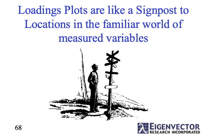
A slide from Chemometrics without Equations explaining PCA in everyday terms.
Don and Neal first presented CWE at the 16th International Forum on Process Analytical Chemistry (IFPAC) in San Diego on January 21-22, 2002. The course was taught hands-on using PLS_Toolbox. CWE was repeated at CPAC’s Summer Institute that July and again at the Federation of Analytical Chemistry and Spectroscopy Societies (FACSS, now SCIX) conference in October 2022 in Ft. Lauderdale, FL. This marked the beginning of CWE’s 20 year run at fall conferences. It was repeated in 2003 at FACSS and in 2004 moved to the Eastern Analytical Symposium (EAS), its home through this year. The workshop has been offered every year, except in 2020 when COVID-19 prevented a physical conference.
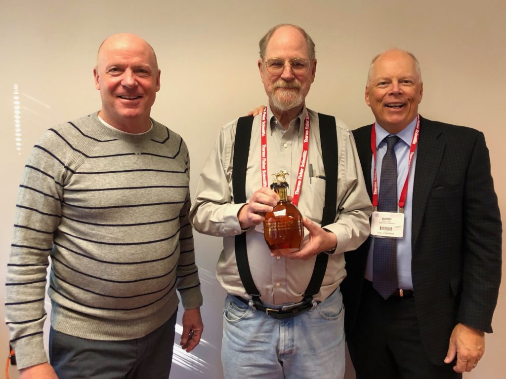
EAS 2022 marks Don’s final presentation of the course at EAS, making a total of 20 fall conference appearances. Each time Don has been assisted by either Neal or myself. Knowing that Don was an avid bourbon connoisseur we commemorated the occasion with a bottle of Blanton’s as he completed his final class.
Neal, Don and Barry celebrating Don’s final Chemometrics without Equations course at Eastern Analytical Symposium.
Looking back on 20 years of teaching CWE Don observed:
EAS has allowed me to meet many scientist who wish to learn and use chemometrics. They have included not only scientists in chemistry, but also those in related fields such as forensic science and cultural heritage. I have had the privilege to offer special versions of the course, tailored to the latter two fields. I have been able to present the course at John Jay College of Criminal Justice, the Forensic Science Department at the University of New Haven, the Museum of Modern Art, the Getty Museum and the Library of Congress. My goal has been to introduce the power of chemometrics to those inside and outside of analytical chemistry. Even though it is time to end my presentations at EAS, I intend to continue to help those who wish to explore the field of chemometrics.
Over 20+ years Professor Dahlberg has gently introduced hundreds to the field of chemometrics with CWE taught at conferences, at in-house classes and online. Thanks Don for your service to field! Cheers and bottoms up!
If you’d like to have Chemometrics without Equations presented at your site, please write bmw@eigenvector.com and we’ll help you arrange it.
There are a number of measures that are used to evaluate the performance of machine learning/chemometric models for calibration, i.e. for predicting a continuous value. Most of these come down to reducing the model error, the difference between the reference values and the values predicted (estimated) by the model, to some single measure of “goodness.” The most ubiquitous measure is the correlation coefficient R2. Many people have produced examples of how data sets can be very different and still produce the same R2 (see for example What is R2 All About?). Those arguments are important but well known and I’m not going to reproduce them here. My main beef with R2 is that it is not in the units that I care about; it is in fact dimensionless. Models used in the chemical domain typically predict values like concentration (moles per liter or weight percent) or some other property value like tensile strength (kilo-newtons per mm2) so it is convenient to have the model error expressed in these terms. That’s why the chemometrics community tends to rely on the measures like root mean square error of calibration (RMSEC). This measure is in the units of the property being predicted.
We also want to know about “goodness” in a number of different circumstances. The first is when the model is being applied to the same data that was used to derive it. This is the error of calibration and we often refer to the calibration R2 or alternately the RMSEC. The second situation is when we are performing cross validation (CV) where the majority of the calibration data set is used to develop the model and then the model is tested on the left out part, generally repeating this procedure until all samples (observations) have been left out once. The results are then aggregated to produce the cross-validation equivalent of R2, which is Q2, or the cross validation equivalent of RMSEC, which is RMSECV. Finally, we’d like to know how models perform on totally independent test sets. For that we use the prediction Q2 and the RMSEP.
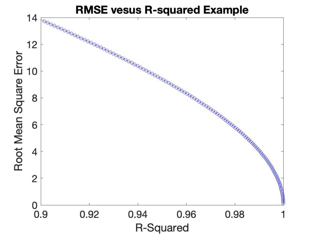
Besides the fact that R2 is not in the same units as the value being predicted, it has a non-linear relationship with it. In the plot below the RMSEC is plotted versus R2 for a synthetic example.
Figure 1: Example of Non-linear Relationship between RMSEC and R2 for a synthetic example.
Overfit is another performance measure of interest. The amount of overfit is the difference between the error of calibration (R2 or RMSEC) and prediction, typically in cross-validation (Q2 or RMSECV). Generally, model error is lower in calibration than in cross validation (or prediction, but that is subject to corruption by prediction test set selection). So a somewhat common plot to make is R2-Q2 versus Q2. (I first saw these in work by David Broadhurst.) An example of such a plot is shown in Figure 2 on the left for a simple PLS model where each point is using a different number of LVs. The problem with this plot is that neither axis is physically meaningful. We know that the best models should somehow be in the lower right corner, but how much difference is significant? And how does it relate to the accuracy with which we need to predict?
Figure 2: Example R2-Q2 versus Q2 plot for a PLS model (left) and RMSECV/RMSEC versus RMSECV (right). Number of PLS latent variables indicated.
I propose here an alternative, which is to plot the ratio of RMSECV/RMSEC versus RMSECV, which is shown in Figure 2 on the right. Now the best model would be in the lower left corner, where the amount of overfit is small along with the prediction error in cross-validation.
Lately I’ve been working with Gray Classical Least Squares (CLS) models, where Generalized Least Squares (GLS) weighting filters are used with CLS to improve performance. Without going into details here (for more info see this presentation) the model can be tuned with a single parameter, g, which governs the aggressiveness of the GLS filter. A data set of NIR spectra of a styrene-butadiene co-polymer system is used as an example (data from Dupont thanks to Chuck Miller). The goal of the model is to predict the weight percent of each of the 4 polymer blocks. The R2-Q2 versus Q2 plot for the four reference concentrations are shown in the left panel of Figure 3 while the corresponding RMSECV/RMSEC versus RMSECV curves are shown the right. The g parameter is varied from 0.1 (least filtering) to 0.0001 (most filtering).
Figure 3: R2-Q2 versus Q2 plot for a GLS-CLS model (left) and RMSECV/RMSEC versus RMSECV (right). Series for each analyte is a function of the GLS tuning parameter g.
As in figure 2 approximately the same information is presented in each plot but the RMSECV/RMSEC plot is more easily interpreted. For instance, the R2-Q2 plot would lead one to believe that the predictions for 1-2-butadiene were quite a bit better than for styrene as their Cross-validation Q2 is substantially better. However, the RMSECV/RMSEC plot shows that the models perform similarly with an RMSECV around 0.8 weight percent. The difference in Q2 for these models is a consequence of the distribution of the reference values and is not indicative of a difference in model quality. The RMSECV/RMSEC shows that the models are somewhat prone to overfitting as this ratio goes to rather high values for aggressive GLS filters. The is less obvious in the R2-Q2 plot as it is not obvious what this difference really relates to in terms of amount of overfitting. And a given change in R2-Q2 is more significant in models with high Q2 than with lower Q2. The R2-Q2 plot would lead one to believe that the 1-2-butadiene model was not overfit much even at g = 0.0001, whereas the styrene model is. In fact, their RMSECV/RMSEC ratio is over 5 for both these models at the g = 0.00001 point, which is terribly overfit.
The RMSECV/RMSEC plot can be further improved if the reference error in the property being predicted is known. In general it is not possible for the apparent model performance to be better than this. Even if the model is predicting the divine omniscient only God knows true answer, the apparent error will still be limited by the error in the reference values. Occasionally models do appear to predict better than the reference error but this is generally a matter of luck. (And yes, it is possible for models to predict better than the reference error, but that is a demonstration for another time.) So it would be useful to add the (root mean square or standard deviation) reference error, if known, as a vertical line.
Based upon the results I’ve seen to date, I highly recommend the RMSECV/RMSEC plot over the R2-Q2 plot for assessing model performance. Model fit and cross-validation metrics are in units of the properties being predicted, and the plots are more linear with respect to changes in these metrics. This plot is easily made for PLS models in PLS_Toolbox and Solo, of course!
The term chemometrics was coined by Svante Wold in a grant application he submitted in 1971 while at the University of Umeå. Supposedly, he thought that creating a new term, (in Swedish it is ‘kemometri’), would increase the likelihood of his application being funded. In 1974, while on a visit to the University of Washington, Svante and Bruce Kowalski founded the International Chemometrics Society over dinner at the Casa Lupita Mexican restaurant. I’d guess that margaritas were involved. (Fun fact: I lived just a block from Casa Lupita in the late 70s and 80s.)
Chemometrics is a good word. The “chemo” part of course refers to chemistry and “metrics” indicates that it is a measurement science: a metric is a meaningful measurement taken over a period of time that communicates vital information about a process or activity, leading to fact-based decisions. Chemometrics is therefore measurement science in the area of chemical applications. Many other fields have their metrics: econometrics, psychometrics, biometrics. Chemical data is also generated in many other fields including biology, biochemistry, medicine and chemical engineering.
So chemometrics is defined as the chemical discipline that uses mathematical, statistical, and other methods employing formal logic to design or select optimal measurement procedures and experiments, and to provide maximum relevant chemical information by analyzing chemical data.
In spite of being a nearly perfect word to capture what we do here at Eigenvector, there are two significant problems encountered when using the term Chemometrics: 1) In spite of the existence of the field for nearly five decades and two dedicated journals (Journal of Chemometrics and Chemometrics and Intelligent Laboratory Systems), the term is not widely known. I still run into graduates of chemistry programs who have never heard the term, and of course it is even less well known in the related disciplines, and less yet in the general population. 2) Many that are familiar with the term think it refers to a collection of primarily projection methods, (e.g. Principal Components Analysis (PCA), Partial Least Squares Regression (PLS)), and therefore other Machine Learning (ML) methods (e.g. Artificial Neural Networks (ANN), Support Vector Machines (SVM)) are not chemometrics regardless of where they are applied. Problem number 2 is exacerbated by the current Artificial Intelligence (AI) buzz and the proclivity of managers and executives towards things that are new and shiny: “We have to start using AI!”
Typical advertisement presented when searching on Artificial Intelligence
This wouldn’t matter much if choosing the right terms wasn’t so critical to being found. Search engines pretty much deliver what was asked for. So you have to be sure you are using terms that are actually being searched on. So what to use?
A common definition of artificial intelligence is the theory and development of computer systems able to perform tasks that normally require human intelligence. This is a rather low bar. Many of the models we develop make better predictions than humans could to begin with. But AI is generally associated with problems such as visual perception and speech recognition, things that humans are particularly adept at. These AI applications generally require very complex deep neural networks etc. And so while you could say we do AI this feels like too much hyperbole, and certainly there are other arguments against using this term loosely.
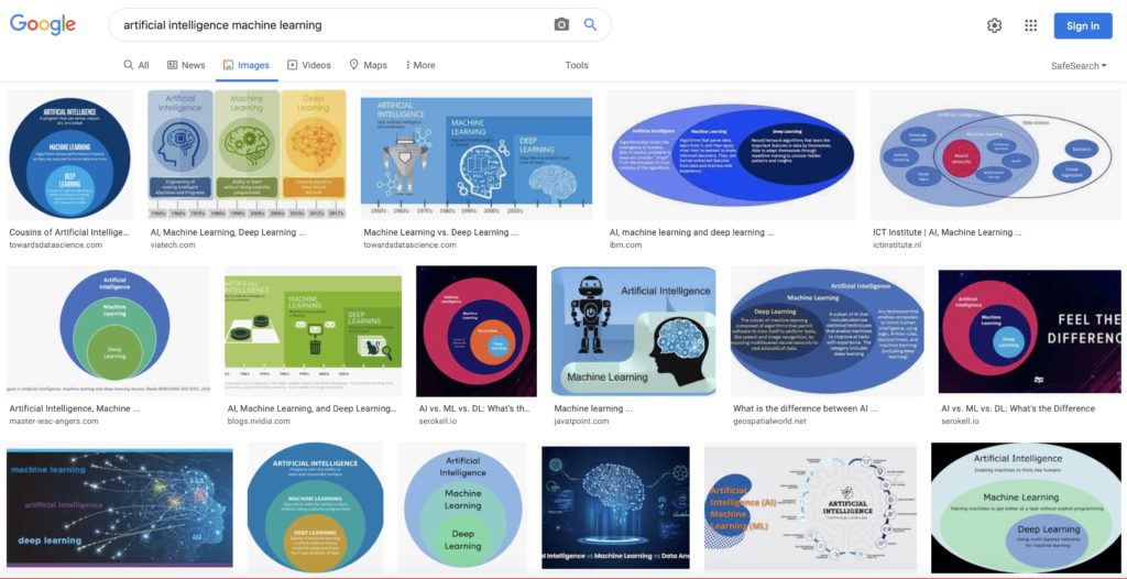
Machine learning is the use and development of computer systems that are able to learn and adapt without following explicit instructions, by using algorithms and statistical models to analyze and draw inferences from patterns in data. Most researchers (apparently) view ML as a subset of AI. Do a search on “artificial intelligence machine learning images” and you’ll find many Venn diagrams illustrating this. I tend to see it as the other way around: AI is the subset of ML that uses complex models to address problems like visual perception. I’ve always had a problem with the term “learning” as it anthropomorphizes data models: they don’t learn, they are parameterized! (If these models really do learn I’m forced to conclude that I’m just a machine made out of meat.) In any case, models from Principal Components Regression (PCR) through XGBoost are commonly considered ML models, so certainly the term machine learning applies to our software.
Google Search on ‘artificial intelligence machine learning’ with ‘images’ selected.
Process analytics is a much less used term and particular to chemical process data modeling and analysis. There are however conferences and research centers that use this term in their name, e.g.IFPAC, APACT and CPACT. Cheminformatics sounds relevant to what we do but in fact the term refers to the use of physical chemistry theory with computer and information science techniques in order to predict the properties and interactions of chemicals.
Data science is defined as the field that uses scientific methods, processes, algorithms and systems to extract knowledge and insights from data. Certainly this is what we do at Eigenvector, but of course primarily in chemistry/chemical engineering where we have a great deal of specific domain knowledge such as the fundamentals of spectroscopy, chemical processes, etc. Thus the term chemical data science describes us pretty well.
So you will find that we will use the terms Machine Learning and Chemical Data Science a lot in the future though we certainly will continue to do Chemometrics!
The development of a machine learning model is typically a fairly involved process, and the software for doing this commensurately complex. Whether it be a Partial Least Squares (PLS) regression model, Artificial Neural Network (ANN) or Support Vector Machine (SVM), there are a lot of calculations to be made to parameterize the model. These include everything from calculation of projections, matrix inverses and decompositions, computing fit and cross-validation statistics, optimization, you name it, it’s in there. Lots of loops and logic and checking convergence criteria, etc.
On the other hand, the application of these models, once developed, is typically quite straight forward. Most models can be applied to new data using a fairly simple recipe involving matrix multiplications, scalings, projections, activation functions, etc. There are exceptions, such as preprocessing methods like iterative Weighted Least Squares (WLS) baselining and models like Locally Weighted Regression (LWR) where you really don’t have a model per se, you have a data set and a procedure. (More on WLS and LWR in a minute!) But in the vast majority of cases effective models can be developed using methods whose predictions can be reduced to simple formulas.
Enter Model_Exporter. When you create any of the models shown at right (key to acronyms below) in PLS_Toolbox or Solo, Model_Exporter can take that model and create a numerical recipe for applying it to new data, including the supported preprocess steps. This recipe can be output in a number of formats, including MATLAB .m, Python .py or XML. And using our freely available Model_Interpreter, the XML file can be incorporated into Java, Microsoft .NET, or generic C# environments.
So what does all this mean?
Total model transportability. Models can be built into any framework you need them in, from process control systems to hand-held analytical instruments.
Minimal footprint. Exported model also have a very small footprint and minimal computing overhead. This means that they can be made to run with minimal memory and computing power.
Order of magnitude faster execution. Lightweight recipe produces predictions much faster than the original model.
Complete transparency. There’s no guessing as to exactly how the model gets from measurements to predictions, it’s all there.
Simplified model validation. Don’t validate the code that makes the model, validate the model!
This is why our customers in many industries, from analytical instrument developers to the chemical process industries, are getting their models online using Model_Exporter. It is creating a revolution in how online models are generated and executed.
And what about those cases like WLS and LWR noted above? We’re working to create add-ons so exported models can utilize these functions too. Look for them, along with some additional model types, in the next release.
Is it for everybody? Well not quite. There are still times where you need a full featured prediction engine like our Solo_Predictor that has built in communication protocols (e.g. socket connections), scripting ability, and can run absolutely any model you can make in PLS_Toolbox or Solo (like hierarchical and even XGBoost). But we’re seeing more and more instances of companies utilizing the advantages of Model_Exporter.
Join the Model_Exporter revolution for the compact, efficient and seamless application of your machine learning models!
BMW
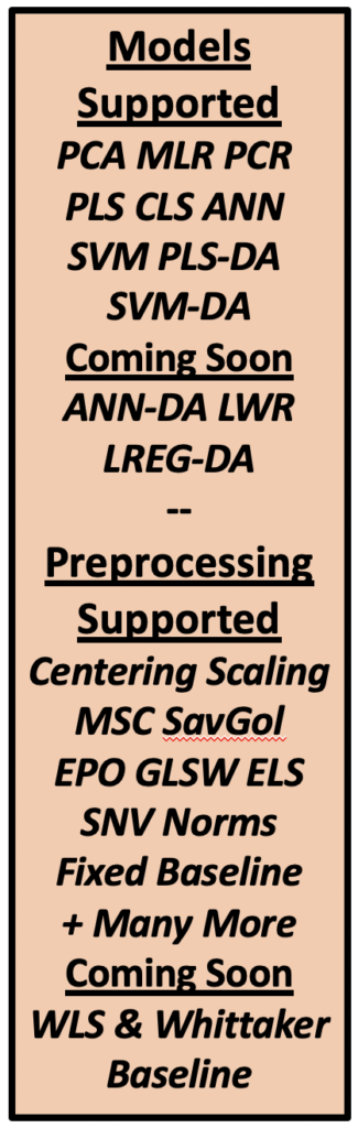
Models Supported: Principal Components Analysis (PCA), Multiple Linear Regression (MLR), Principal Components Regression (PCR), Partial Least Squares Regression (PLS), Classical Least Squares (CLS), Artificial Neural Networks (ANN), Support Vector Machine Regression (SVM), Partial Least Squares Discriminant Analysis (PLS-DA), Support Vector Machine Discriminant Analysis (SVM-DA), Artificial Neural Network Discriminant Coming Soon: Analysis (ANN-DA), Locally Weighted Regression (LWR), Logistic Regression Discriminant Analysis (LREG-DA).
Preprocessing Methods Supported: General scaling and centering options including Mean and Median Centering, Autoscaling, Pareto and Poisson Scaling, Multiplicative Scatter Correction (MSC), Savitsky-Golay Smoothing and Derivatives, External Parameter Orthogonalization (EPO), Generalized Least Squares Weighting (GLSW), Extended Least Squares, Standard Normal Variate (SNV), 1-, 2-, infinity and n-norm Normalization, Fixed point spectral baselining. Coming Soon: Iterative Weighted Least Squares Baselining (WLS) and Whittaker Baslining.
I’ve followed this story a bit since first hearing of Theranos and their claims to be able to run hundreds of blood tests simultaneously on just a few drops of blood. Based on my experience this seemed more than unlikely. At Eigenvector we’ve worked on quite a few medical device development projects. This includes projects involving atherosclerotic plaques, cervical cancer, muscle tissue oxygenation, burn wound healing, limb ischemia, non-invasive glucose monitoring, non-invasive blood alcohol estimation and numerous other projects involving blood and urine tests. So we’ve developed an appreciation of how hard it is to develop new analytical techniques on biological samples. Beyond that, we’ve also learned a lot about the error in the reference methods we were trying to match. Even under ideal conditions, with standard laboratory equipment and large sample volumes, results are far from perfect.
So when the whole thing was blown wide open by Carreyrou’s reports in the Wall Street Journal I wasn’t surprised. I read several of the follow up articles as well. But as one reviewer of the book said, “No matter how bad you think the Theranos story was, you’ll learn that the reality was actually far worse.” I’ll say. Honestly it took me a while to get into the book, in fact, I put it down for a month because it just made me so mad.
We’ve had a few consulting clients over the years that were, let’s say, overly enthusiastic. To varying degrees some of them have been unrealistic about the robustness of their technology and have failed to address problems that could potentially impact accuracy. (I’m happy to report that none of our current consulting clients fall into this category.) In some instances things we saw as potential show stoppers were simply declared non-problems. In other cases people abused the data including cherry picking and grossly overfit and non-validated models. (My favorite line was when one client’s lawyer told me I didn’t know how to use my own software.) We have had falling outs with some of these folks when our analysis didn’t support their contentions.
But none of the people we’ve dealt with approached the level of overselling their technology to the degree that Holmes took it. As I see it there are two reasons for this. The first is that Holmes is a sociopath. Carreyrou said he would leave it to others to make that assessment but it seems obvious to me. Maybe she didn’t start out that way, but it’s clear that very early on she started believing her own bullshit. Defending that belief became all that mattered. And she teamed with Ramesh “Sunny” Balwani who was if anything worse. They ran an organization that was based on secrecy, lies and intimidation. And they made sure that nobody on their board had the scientific background to question the feasibility of what they were claiming they’d do.
But the second reason they got as far as they did was because they were exceedingly well connected. The book identifies these connections but doesn’t really discuss them in terms of being enablers of the scam that ensued. It started with Elizabeth’s parents connections to people around Stanford, and Elizabeth’s ChemE professor at Stanford, Channing Robertson. These lead to funding and legal help. From there Holmes just played leapfrog with these connections ending at former secretary of State George Shultz, (who I learned actually lives on the Stanford campus) and his circle including Henry Kissinger, James Mattis and high profile lawyer David Boies. (Boies led the Justice Department’s anti-trust suit against Microsoft, and was Al Gore’s lawyer in he 2000 election.) Famous for his scorched earth tactics, Boies and his firm kept the lid on things at Theranos by threatening lawsuits against potential whistleblowers and further intimidating them by hiring private eyes to surveil them. Having no firmer grasp of the science and engineering realities of what Theranos was attempting than the board members, Boies’ firm did this in exchange for stock options.
It’s second point here that really bothers me. There will always be people like Holmes that are willing to ignore the damage that they may do to others while pursuing wealth or fame and fortune. But this behavior was enabled by well-heeled and well-connected people that failed completely on their due diligence obligations from financial, scientific and most importantly, medical ethics perspectives. Somehow they completely forgot Carl Sagan’s adage “extraordinary claims require extraordinary evidence.” It’s hard to imagine that this could have ever gotten so far out of hand had Holmes attended a state university and had unconnected parents. Investors to whom you are not connected and who are not so wealthy as to be able to afford to lose a lot of money have a much higher standard of proof.
In our consulting capacity at Eigenvector we always try to be optimistic about what’s possible, and we do our best to help clients achieve success. But we never pull our punches with regards to the limitations of the technology we’re working with and the models we develop based on the data it produces. Theranos produced millions of inaccurate blood tests that were eventually vacated. While it doesn’t appear that anybody actually died because of these inaccurate tests, they certainly caused a lot of anxiety, lost time and expense among the customers. It’s our pledge that we will always do our due diligence, and expect those around us to do the same, so that Eigenvector will never be part of a fiasco like this.
I’ve just returned from Conference Chimiométrie 2020, the annual French language chemometrics conference, now in its 21st edition. The conference was held in Liège and unfortunately there wasn’t much time to explore the city. I can tell you they have a magnificent train station, Gare de Liège is pictured at right.
The vibrant French chemometrics community always produces a great conference with good attendance, well over 120 at this event, and food and other aspects were as enjoyable as ever thanks to the local organizing committee and conference chair Professor Eric Ziemons.
Age Smilde got the conference off to a good start with “Common and Distinct Components in Data Fusion.” In it he described a number of different model forms, all related to ANOVA Simultaneous Components Analysis (ASCA), for determining if the components in different blocks of data are unique or shared. What struck me most about this talk and many of the ones that followed is that there are a lot of different models out there. As Age says, “Think about the structure of your data!” The choice of model structure is critical to answering the questions posed to the data. And it is only with solid domain knowledge that appropriate modeling choices are made.
In addition to a significant number of papers on multi-block methods, Chimiométrie included quite a few papers in the domain of metabolomics, machine learning, Bayesian methods, and a large number of papers on hyper spectral image analysis (see the Programme du Congrès). All in all, a very well rounded affair!
I was pleased to see a good number of posters that utilized our PLS_Toolbox and in some instances MIA_Toolbox software very well! The titles are given below with links to the posters. We’re always happy to help researchers achieve an end result or provide a benchmark towards the development of new methods!
A colleague wrote to me recently and asked if Eigenvector was considering rebranding itself as a Data Science company. My knee-jerk response was “isn’t that what we’ve been for the last 25 years?” But I know exactly what she meant: few people have heard of Chemometrics but everybody has heard about Data Science. She went on to say “I am spending increasing amounts of time calming over-excited people about the latest, new Machine Learning (ML) and Artificial Intelligence (AI) company that can do something slightly different and better…” I’m not surprised. I know it’s partly because Facebook and LinkedIn have determined that I have an interest in data science, but my feeds are loaded with ads for AI and ML courses and data services. I’m sure many managers subscribe to the Wall Street Journal’s “Artificial Intelligence Daily” and, like the Stampeders on Chilkoot Pass pictured below, don’t want to miss out on the promised riches.
Oh boy. Déjà vu. In the late 80s and 90s during the first Artificial Neural Network (ANN) wave there were a slew of companies making similar promises about the value they could extract from data, particularly historical/happenstance process data that was “free.” One slogan from the time was “Turn your data into Gold.” It was the new alchemy. There were successful applications but there were many more failures. The hype eventually faded. One of biggest lessons learned: Garbage In, Garbage Out.
I attended The MathWorks Expo in San Jose this fall. In his keynote address, “Beyond the ‘I’ in AI,” Michael Agostini stated that 80-90% of the current AI initiatives are failing. The main reason: lack of domain knowledge. He used as an example the monitoring of powdered milk plants in New Zealand. The moral of the story: you can’t just throw your data into a ML algorithm and expect to get out anything very useful. Perhaps tellingly, he showed plots from Principal Components Analysis (PCA) that helped the process engineers involved diagnose the problem, leading to a solution.
Another issue involves what sort of data is even appropriate for AI/ML applications. In the early stages of the development of new analytical methods, for instance, it is common to start with tens or hundreds of samples. It’s important to learn from these samples so you can plan for additional data collection: that whole experimental design thing. And in the next stage you might get to where you have hundreds to thousands of samples. The AI/ML approach is of limited usefulness In this domain. First off it is hard to learn much about the data using these approaches. And maintaining parsimony is challenging. Model validation is paramount.
The old adage “try simple things first” is still true. Try linear models. Use your domain knowledge to select sample sets and variables, and to select data preprocessing methods that remove extraneous variance from the problems. Think about what unplanned perturbations might be affecting your data. Plan on collecting additional data to resolve modeling issues. The opposite of this approach is what we call the “throw the data over the wall” model where people doing the data modeling are separate from the people who own the data and the problem associated with it. Our experience is that this doesn’t work very well.
There are no silver bullets. In 30 years of doing this I have yet to find an application where one and only one method worked far and away better than other similar approaches. Realize that 98% of the time the problem is the data.
So is Eigenvector going to rebrand itself as a Data Science company? We certainly want people to know that we are well versed in the application of modern ML methods. We have included many of these tools in our software for decades, and we know how to work with these methods to obtain the best results possible. But we prefer to stay grounded in the areas where we have domain expertise. This includes problems in spectroscopy, analytical chemistry, chemical process monitoring and control. We all have backgrounds in chemical engineering, chemistry, physics, etc. Plus collectively over 100 man-years experience developing solutions that work with real data. We know a tremendous amount about what goes wrong in data modeling and what approaches can be used to fix it. That’s where the gold is actually found.
Eigenvector Research, Inc. was founded on January 1, 1995 by myself and Neal B. Gallagher, so we’re now 25 years old. On this occasion I feel that I should write something though I’m at a bit of loss with regards to coming up with a significantly profound message. In the paragraphs below I’ve written a bit of history (likely overly long).
PLS_Toolbox Floppy Disks 1994-1997
We started Eigenvector with each of us buying a Power Mac 8100 with keyboard, mouse and monitor. These were about $4k, plus another $1700 to upgrade the 8Mb RAM it came with to 32Mb. Liz Callanan at The MathWorks gave us our first MATLAB licenses-thanks! PLS_Toolbox was in version 1.4 and still being marketed under Eigenvector Technologies. Our founding principle was and still is:
Life is too short to drink bad beer, do boring work or live in a crappy place.
That’s a bit tongue-in-cheek but it’s basically true. We certainly started Eigenvector to keep ourselves in interesting work. For me that meant continuing with chemometrics, data analysis in chemistry. New data sets are like Christmas presents, you never know what you’ll find inside. For Neal I think it meant anything you could do that let you use math on a daily basis. Having both grown up in rural environments and being outdoor enthusiasts location was important. And the bit about beer is just, well, duh!
As software developers we found it both interesting and challenging to make tools that allowed users (and ourselves!) to build successful models for calibration, classification, MSPC etc. As consultants we found a steady stream of projects which required both use of existing chemometric methods and adaptation of new ones. As we became more experienced we learned a great deal about what can make models go bad: instrument drift, differences between instruments, variable and unforeseen background interferents, etc. and often found ourselves as the sanity check to overly optimistic instrument and method developers. Determining what conclusions are supportable given the available data remains an important function for us.
Our original plan included only software and consulting projects but we soon found out that there was a market for training. (This seems obvious in retrospect.) We started teaching in-house courses when Pat Wiegand asked us to do one at Union Carbide in 1996. A string of those followed and soon we were doing workshops at conferences. And then another of our principles kicked in:
Let’s do something, even if it’s wrong.
Neal Teaching Regression at EigenU
Entrepreneurs know this one well. You can never be sure that any investment you make in time or dollars is actually going to work. You just have to try it and see. So we branched out into doing courses at open sites with the first at Illinois Institute of Technology (IIT) in 1998, thanks for the help Ali Çinar! Open courses at other sites followed. Eigenvector University debuted at the Washington Athletic Club in Seattle in 2006. We’re planning the 15th Annual EigenU for this spring. The 10th Annual EigenU Europe will be in France in October and our third Basic Chemometrics PLUS in Tokyo in February. I’ve long ago lost count of the number of courses we’ve presented but it has to be well north of 200.
Our first technical staff member, Jeremy M. Shaver, joined us in 2001 and guided our software development for over 14 years. Our collaborations with Rasmus Bro started the next year in 2002 and continue today. Initially focused on multi-way methods, Rasmus has had a major impact on our software from numerical underpinnings to usability. Our Chemometrics without Equations collaboration with Donald Dahlberg started in 2002 and has been taught at EAS for 18 consecutive years now.
So what’s next? The short answer: more of the same! It’s both a blessing and a curse that the list of additions and improvements that we’d like to make to our software is never ending. We’ll work on that while we continue to provide the outstanding level of support our users have come to expect. Our training efforts will continue with our live courses but we also plan more training via webinar and in other venues. And of course we’re still doing consulting work and look forward to new and interesting projects in 2020.
In closing, we’d like to thank all the great people that we’ve worked with these 25 years. This includes our staff members past and present, our consulting clients, academic colleagues, technology partners, short course students and especially the many thousands of users of our PLS_Toolbox software, its Solo derivatives and add-ons. We’ve had a blast and we look forward to continuing to serve our clients in the new decade!
I attended Metabolomics 2019 and was pleased to find a rapidly expanding discipline populated with very enthusiastic researchers. Applications ranged from developing plants with increased levels of nutrients to understanding cancer metabolism.
Metabolomics experiments, however, produce extremely large and complex data sets. Consequently, the ultimate success of any experiment in metabolomics hinges on the software used to analyze the data. It was not surprising to find that multivariate analysis methods were front and center in many of the presentations and posters.
At the conference I saw some nice examples using our software, but of course not as many as I would have liked. So when I got home I put together this table comparing our PLS_Toolbox and Solo software with SIMCA, R and Python for use with metabolomics data sets.
Compare Software for Metabolomics
PLS_Toolbox
Solo
SIMCA
R/Python
Available for Windows,
Mac and Linux?
Yes
Yes
Windows only
Yes
Comes with User Support?
Yes
Yes
Yes
No
Point-and-click GUIs for
all important analyses?
Yes
Yes
Yes
No
Command Line available?
Yes
No
No
Yes, use is mandatory
Source Code available
for review?
Yes
Yes, same
code as
PLS_Toolbox
No
Yes
Includes PCA, PLS, O-PLS?
Yes
Yes
Yes
Add-ons available
Includes ASCA, MLSCA?
Yes
Yes
No
Add-ons available
Includes SVMs, ANNs
and XGBoost?
Yes
Yes
No
Add-ons available
Includes PARAFAC,
PARAFAC2, N-PLS?
Yes
Yes
No
Add-ons available
Includes Curve Resolution Methods?
Yes
Yes
No
Add-ons available
Extensible?
Yes
No
Yes, through Python
Yes
Instrument standardization,
calibration transfer tools?
Yes
Yes
No
No
Comes complete?
Yes
Yes
Yes
No
Easy to install?
Yes
Yes
Yes
No
Cost
Inexpensive
Moderate
Expensive
Free
So it’s easy to see that PLS_Toolbox is in the sweet spot with regards to metabolomics software. Yes, it requires MATLAB, but MATLAB has over 3 millions users and is licensed by over 5000 universities world wide. And if you don’t care to use a command line Solo includes all the tools in PLS_Toolbox and doesn’t require MATLAB. Plus, Solo and PLS_Toolbox share the same model and data formats. So you can have people in your organization that use only GUIs work seamlessly with people who prefer access to the command line.
So the bottom line here is:
If you are just getting started with metabolomics data PLS_Toolbox and Solo are easy to install, include all the analysis tools you’ll need in easy to use GUIs, are transparent and are relatively inexpensive.
If you are using SIMCA, you should try out PLS_Toolbox because it includes many methods that SIMCA doesn’t have, the source code is available, its more easily extensible, works on all platforms, and it will save you money.
If you are using R or Python, you should consider PLS_Toolbox because it is fully supported by our staff, has all the important tools in one place, sophisticated GUIs, and is easy to install.
Ready to try PLS_Toolbox or Solo? Start by creating an account and you’ll have access to free fully functional demos. Questions? Write to me!
Chimiométrie 2019 was held in Montpellier, January 30 to February 1. Now in its 20th year the conference attracted over 150 participants. The conference is mostly in French, (which I have been trying to learn for many years now), but also with talks in English. The Scientific and Organizing Committee Presidents were Ludovic Duponchel and J.M. Roger, respectively.
Eigenvector was proud to sponsor this event, and it was fun to have a display table and a chance to talk with some of our software users in France. As usual, I was on the lookout for talks and posters using PLS_Toolbox. I especially enjoyed the talk presented by Alice Croguennoc, Some aspects of SVM Regression: an example for spectroscopic quantitative predictions. The talk provided a nice intro to Support Vectors and good examples of what the various parameters in the method do. Alice used our implementation of SVMs, which adds our preprocessing, cross-validation and point-and-click graphics to the publicly available LIBSVM package. Ms. Croguennoc demonstrated some very nice calibrations on a non-linear spectroscopic problem.
I also found three very nice posters which utilized PLS_Toolbox:
Preliminary appreciation biodegradation of formate and fluorinated ethers by means of Raman spectroscopy coupled with chemometrics by M. Marchetti, M. Offroy, P. Bourson, C. Jobard, P. Branchu, J.F. Durmont, G. Casteran and B. Saintot.
By all accounts the conference was a great success, with many good talks and posters covering a wide range of chemometric topics, a great history of the field by Professor Steven D. Brown, and a delicious and fun Gala dinner at the fabulous Chez Parguel, shown at left. The evening included dancing, and also a song, La Place De la Conférence Chimiométrie, (sung to the tune of Patrick Bruel’s Place des Grands Hommes), written by Sylvie Roussel in celebration of the conference’s 20th year and sung with great gusto by the conferees. Also, the lecture hall on the SupAgro campus was very comfortable!
Congratulations to the conference committees for a great edition of this French tradition, with special thanks to Cécile Fontange and Sylvie Roussel of Ondalys for their organizational efforts. À l’année prochaine!
I logged in to LinkedIn this morning and found a discussion about Python that had a lot of references to PLS_Toolbox in it. The thread was started by one of our long time users, Erik Skibsted who wrote:
“MATLAB and PLS_Toolbox has always been my preferred tools for data science, but now I have started to play a little with Python (and finalised my first on-line course on Data Camp). At Novo Nordisk we have also seen a lot of small data science initiatives last year where people are using Python and I expect that a lot more of my colleagues will start coding small and big data science projects in 2019. It is pretty impressive what you can do now with this open source software and different libraries. And I believe Python will be very important in the journey towards a general use of machine learning and AI in our company.”
This post prompted well over 20 responses. As creator of PLS_Toolbox I thought I should jump in on the discussion!
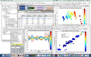
In his response, Matej Horvat noted that Python and other open source initiatives were great “if you have the required coding skills.” This a key phrase. PLS_Toolbox doesn’t require any coding skills _at all_. You can use it entirely in point-and-click mode and still get to 90% of what it has to offer. (This makes it the equivalent of using our stand-alone product Solo.) When you are working with PLS_Toolbox interfaces it looks like the first figure below.
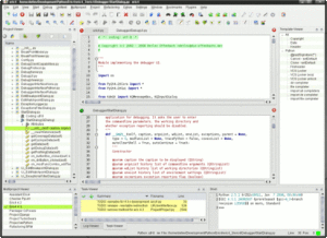
Of course if you are a coder you can take advantage of the ability to also use it in command line mode and build it into your own scripts and functions, just like you would do with other MATLAB toolboxes. The caveat is that you can’t redistribute it without an additional license from us. (We do sell these of course, contact me if you are interested.) When you are working with Python, (or developing MATLAB scripts incorporating PLS_Toolbox functions for that matter), it looks like the second figure.
Like Python, PLS_Toolbox is “open source” in the sense that you can actually see the code. We’re not hiding anything proprietary in it. You can find out exactly how it works. You can also modify if you wish, just don’t ask for help once you do that!
Unlike typical open source projects, with PLS_Toolbox you also get user support. If something doesn’t work we’re there to fix it. Our helpdesk has a great reputation for prompt responses that are actually helpful. That’s because the help comes from the people that actually developed the software.
Another reason to use PLS_Toolbox is that we have implemented a very wide array of methods and put them into the same framework so that they can be evaluated in a consistent way. For instance, we have PLS-DA, SVM-C, and now XGBoost all in the same interface that use the exact same preprocessing and are all cross-validated and validated in the same exact way so that they can be compared directly.
If you want to be able to freely distribute the models you generate with PLS_Toolbox we have have a tool for that: Model_Exporter. Model_Exporter allows users to export the majority of our models as code that you can compile into other languages, including direct export of Python code. You can then run the models anywhere you like, such as for making online predictions in a control system or with handheld spectrometers such as ThermoFisher’s Truscan. Another route to online predictions is using our stand-alone Solo_Predictor which can run any PLS_Toolbox/Solo model and communicates using a number of popular protocols.
PLS_Toolbox is just one piece of the complete chemometrics solutions we provide. We offer training at our renowned Eigenvector University and many other venues such as the upcoming course in Tokyo, EigenU Online, and an extensive array of help videos. And if that isn’t enough we also offer consulting services to help you develop and implement new instruments and applications.
So before you spend a lot of valuable time developing applications in Python, make sure you’re not just recreating tools that already exist at Eigenvector!
The 13th Annual Eigenvector University was held April 29-May 4 in Seattle. It was a busy, vibrant week with 40 students with a wide variety of backgrounds attending along with 10 instructors. Users of our PLS_Toolbox and Solo chemometrics packages showed some of their recent results at the Wednesday evening poster session, which has become an EigenU tradition. Now combined with our PowerUser Tips & Tricks session, it makes for a full evening of scientific and technical exchange fueled by hors d’oeuvres and adult beverages.
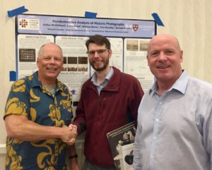
This year’s best poster, (as judged by the EVRI staff), was “Nondestructive Analysis of Historic Photographs” by Arthur McClelland, Elena Bulat, Melissa Banta, Erin Murphy, and Brenda Bernier. The poster described how Specular Reflection FTIR was used with Principal Components Analysis (PCA) to discriminate between coatings applied to prints in the Harvard class albums from 1853-1864.
For his efforts Arthur took home a pair of Bose Soundsport Wireless Headphones. Arthur is shown above accepting his prize from Eigenvector President Barry M. Wise and Vice-president Neal B. Gallagher. Congratulations Arthur!
The runner up poster was “Analytical Approach to Investigate Salt Disproportionation in Tablet Matrices by Stimulated Raman Scattering Microscopy” by Benjamin Figueroa, Tai Nguyen, Yongchao Su, Wei Xu, Tim Rhodes, Matt Lamm, and Dan Fu. The poster demonstrates how the the conversion of Active Pharmaceutical Ingredient (API) from its active salt form to its inactive free base form can be quantified in Raman images of tablets. Benjamin received a Bose Soundlink Bluetooth Speaker for his contribution. Kudos Benjamin!
We were also pleased to have several other very interesting poster submissions, as shown below:
Yulan Hernandez, Lesly Lagos and Betty C. Galarreta, “Selective and Efficient Mycotoxin Detection with Nanoaptasensors using SERS and Multivariate Analysis.”
Devanand Luthria and James Harnly, “Applications of Spectral Fingerprinting and Multivariate Analysis in Agricultural Sciences.”
Thanks to all EigenU 2018 poster presenters for a fun and informative evening!
Integration of Eigenvector’s multivariate analysis software with Metrohm’s Vis-NIR analyzers will give users access to advanced calibration and classification methods.
Metrohm’s spectroscopy software Vision Air 2.0 supports prediction models created in EVRI’s PLS_Toolbox and Solo software and offers convenient export and import functionality to enable measurement execution and sample analysis in Metrohm’s Vision Air software. Customers will benefit from data transfer between PLS_Toolbox/Solo and Vision Air and will enjoy a seamless experience when managing models and using Metrohm’s NIR laboratory instruments. Metrohm has integrated Eigenvector’s prediction engine, Solo_Predictor, so that users can apply any model created in PLS_Toolbox/Solo.
Data scientists, researchers and process engineers in a wide variety of industries that already use or would like to use Eigenvector software will find this solution appealing. PLS_Toolbox and Solo’s intuitive interface and advanced visualization tools make calibration, classification and validation model building a straightforward process. A wide array of model types, preprocessing methods and the ability to create more complex model forms, such as hierarchical models with conditional branches, make Eigenvector software the preferred solution for many.
“This a win-win for users of Metrohm NIR instruments and users of Eigenvector chemometrics software” says Eigenvector President Dr. Barry M. Wise. “Thousands of users of EVRI software will be able to make models for use on Metrohm NIR instruments in their preferred environment. And users of Metrohm NIR instruments will have access to more advanced data modeling techniques.”
Researchers benefit from Metrohm’s Vis-NIR Instrument and Vision Air software through instruments covering the visible and NIR wavelength range, intuitive operation, state-of-the art user management with strict SOPs and global networking capabilities. Combining the solutions will create an integrated experience that will save time, improve product development process and provide better control of product quality.
Key Advantages PLS_Toolbox/Solo:
Integration of Solo_Predictor allows users to run any model developed in PLS_Toolbox/Solo
Allows users to make calibration and classification models in PLS_Toolbox and Solo’s user-friendly modeling environment
Supports standard model types (PCA, PLS, PLS-DA, etc.) with wide array of data preprocessing methods
Advanced models (SVMs, ANNs, etc.) and hierarchical models also supported
Key Advantages Vision Air:
Intuitive workflow due to appealing and smart software concept with specific working interfaces for routine users, and lab managers
Database approach for secure data handling and easy data management
Powerful network option with global networking possibility and one-click instruments maintenance
The ICNIRS conference was held June 11-15 in Copenhagen, Denmark, where close to 500 colleagues gathered for the largest forum on Near-Infared Spectroscopy in the world. The conference featured several keynote lectures, classes taught by EVRI associate Professor Rasmus Bro, and also held several poster sessions where over 20 conference attendees displayed their research using EVRI software! We’d like to feature some of the posters and authors below: thanks for using our software, everyone!
Last month I had the pleasure of attending Chimiométrie XVII. This installment ran from January 17-20 in the beautiful city of Namur, BELGIUM. The conference was largely in French but with many talks and posters in English. (My French is just good enough that I can get the gist of most of the French talks if the speakers put enough text on their slides!) There were many good talks and posters demonstrating a lot of chemometric activity in the French speaking world.
EVRI was also proud to sponsor the poster contest which was won by Juan Antonio Fernández Pierna et al. with “Chemometrics and Vibrational Spectroscopy for the Detection of Melamine Levels in Milk.” For his efforts Juan received licenses for PLS_Toolbox and MIA_Toolbox. Congratulations! We wish him continued success in his chemometric endeavors!
Finally I’d like to thank the organizing committee, headed by Pierre Dardenne of Le Centre wallon de Recherches agronomiques. The scientific content was excellent and, oh my, the food was fantastic! I’m already looking forward to the next one!
On October 1, 1985 I walked into Bruce Kowalski’s chemometrics class and my world changed forever. It was my first day of chemical engineering graduate school at the University of Washington. My M.S. thesis advisor, Prof. Harold Hager, told me that I’d probably find the methods in Bruce’s class useful in treating the data I was to collect. He was right, but more than that, it wasn’t long before I knew that I’d found something I wanted to do for a living.
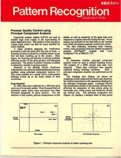
A big part of the class was a project, due at the end of the semester in early December. I spent my Thanksgiving vacation working with Infometrix’s Ein*Sight software doing PCA on data from a Liquid-Fed Ceramic Melter I’d worked on at Pacific Northwest National Laboratory. Ein*Sight had a limit of 100 samples and 10 variables but it ran on an IBM AT. I spent a lot of time swapping interesting samples in and out of the analysis and trying to interpret the results. I got an A on the project (Bruce gave lots of A’s!) and my study became a piece of Infometrix sales literature (left). From there I started working with Prof. Larry Ricker on my ChemE Ph.D. with Bruce on my committee. The rest, as they say, is history.
I always liked data analysis. As an undergrad in ChemE my lab partners referred to me as the “Data Magician.” I just liked massaging the numbers to see what I could tease out. Chemometrics gave me a whole new set of tools and opened my world up to high dimension data.
Chemometrics has taken me lots of interesting places over the last 30 years, and I mean that both with regards to the travel and the intellectual challenges. And I’ve been blessed to meet lots of great people. It’s awesome to go to a conference in a faraway place and walk into a room full of friends.
Thanks to all my friends and colleagues for a great 30 year adventure! But, man!, that was fast! Where did the time go? But I’m looking forward to a couple more decades of chemometrics escapades.
BMW
×
We're transitioning to a new login system. You will be required to reset your password the first time you log into the new system. Please contact us at helpdesk@eigenvector.com if you have any trouble accessing your account.
We use cookies to ensure that we give you the best experience on our website. If you continue to use this site we will assume that you are happy with it.OkNo
 SEARCH


 On the other hand, the application of these models, once developed, is typically quite straight forward. Most models can be applied to new data using a fairly simple recipe involving matrix multiplications, scalings, projections, activation functions, etc. There are exceptions, such as preprocessing methods like iterative Weighted Least Squares (WLS) baselining and models like Locally Weighted Regression (LWR) where you really don’t have a model per se, you have a data set and a procedure. (More on WLS and LWR in a minute!) But in the vast majority of cases effective models can be developed using methods whose predictions can be reduced to simple formulas.
  I’ve just returned from Conference Chimiométrie 2020, the annual French language chemometrics conference, now in its 21st edition. The conference was held in Liège and unfortunately there wasn’t much time to explore the city. I can tell you they have a magnificent train station, Gare de Liège is pictured at right.
 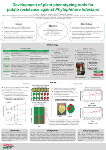 Development of plant phenotyping tools for potato resistance against Phytophthora infestans by François Stevens et. al.
  Oh boy. Déjà vu. In the late 80s and 90s during the first Artificial Neural Network (ANN) wave there were a slew of companies making similar promises about the value they could extract from data, particularly historical/happenstance process data that was “free.” One slogan from the time was “Turn your data into Gold.” It was the new alchemy. There were successful applications but there were many more failures. The hype eventually faded. One of biggest lessons learned: Garbage In, Garbage Out.
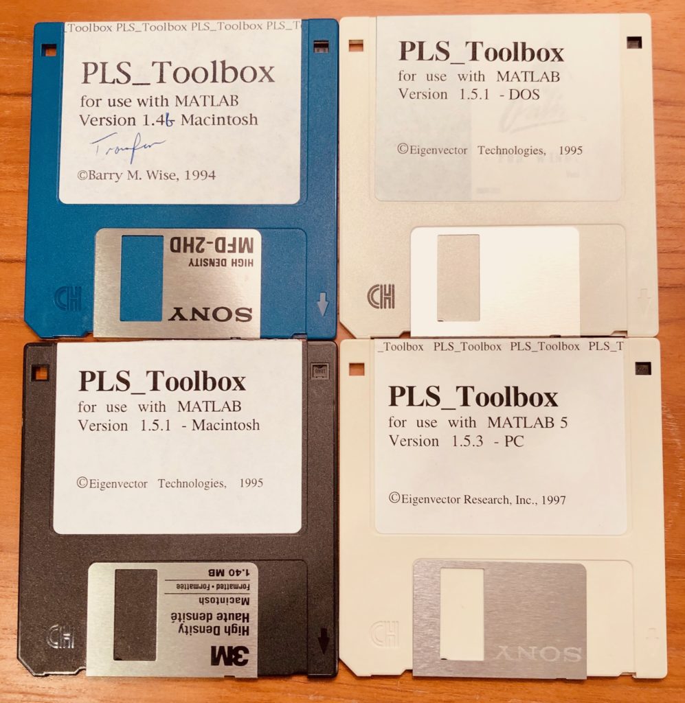
