Category Archives: Software

Scott Ramos of Infometrix wrote me last week and noted that he had followed the discussion on the accuracy of PLS algorithms. Given that they had done considerable work comparing their BIDIAG2 implementation with other PLS algorithms, he was “surprised” with my original post on the topic. He was kind enough to send me a MATLAB implementation of the PLS algorithms included in their product Pirouette for inclusion in my comparison.

Below you’ll find a figure that compares regression vectors from NIPALS, SIMPLS, DSPLS and the BIDIAG2 code provided by Scott. The figure was generated for a tall-skinny X-block (our “melter” data) and for a short-fat X-block (NIR of pseudo-gasoline mixture). Note that I used our SIMPLS and DSPLS that include re-orthogonalization, as that is now our default. While I haven’t totally grokked Scott’s code, I do see where it includes an explicit re-orthogonalization of the scores as well.

Note that all the algorithms are quite similar, with the biggest differences being less than one part in 10¹⁰. The BIDIAG2 code provided by Scott (hot pink with stars) is the closest to NIPALS for the tall skinny case, while being just a little more different than the other algorithms for the short fat case.

This has been an interesting exercise. I’m always surprised when I find there is still much to learn about something I’ve already been thinking about for 20+ years! It is certainly a good lesson in watching out for numerical accuracy issues, and in how accuracy can be improved with some rather simple modifications.

BMW

Version 6.0 of PLS_Toolbox, Solo and Solo+MIA will be out this fall. There will be lots of new features, but right at the moment I’m having fun playing with one in particular: the Analysis Report Writer (ARW). The ARW makes documenting model development easy. Once you have a model developed, just make the plots you want to make, then select Tools/Report Writer in the Analysis window. From there you can select HTML, or if you are on a Windows PC, MS Word or MS Powerpoint for saving your report. The ARW then writes a document with all the details of your model, along with copies of all the figures you have open.

As an example, I’ve developed a (quick and dirty!) model using the tablet data from the IDRC shootout in 2002. The report shows the model details, including the preprocessing and wavelength selection, along with the plots I had up. This included the calibration curve, cross-validation plot, scores on first two PCs, and regression vector. But it could include any number and type of plots as desired by the user. Statistics on the prediction set are also included.

Look for Version 6.0 on our web site in October, or come visit us at FACSS, booth 48.

BMW

Thanks to everybody that responded to the last post on Accuracy of PLS Algorithms. As I expected, it sparked some nice discussion on the chemometrics listserv (ICS-L)!

As part of this discussion, I got a nice note from Klaas Faber reminding me of the short communication he wrote with Joan Ferré, “On the numerical stability of two widely used PLS algorithms.” [1] The article compares the accuracy of PLS via NIPALS and SIMPLS as measured by the degree to which the scores vectors are orthogonal. It finds that SIMPLS is not as accurate as NIPALS, and suggests adding a re-orthogonalization step to the algorithms.

I added re-orthogonalization to the code for SIMPLS, DSPLS, and Bidiag2 and ran the tests again. The results are shown below. Adding this to Bidiag2 produces the most dramatic effect (compare to figure in previous post), and improvement is seen with SIMPLS as well. Now all of the algorithms stay within ~1 part in 10¹² of each other through all 20 LVs of the example problem. Reconstruction of X from the scores and loadings (or weights, as the case may be!) was improved as well. NIPALS, SIMPLS and DSPLS all reconstruct X to within 3e-16, while Biadiag2 comes in at 6e-13.

The simple fix of re-orthogonalization makes Bidiag2 behave acceptably. I certainly would not use this algorithm without it! Whether to add it to SIMPLS is a little more debatable. We ran some tests on typical regression problems and found that the difference on predictions with and without it was typically around 1 part in 10⁸ for models with the correct number of LVs. In other words, if you round your predictions to 7 significant digits or less, you’d never see the difference!

That said, we ran a few tests to determine the effect on computation time of adding the re-orthogonalization step to SIMPLS. For the most part, the effect was negligible, less than 5% additional computation time for the vast majority of problem sizes and at worst a ~20% increase. Based on this, we plan to include re-orthogonalization in our SIMPLS code in the next major release of PLS_Toolbox and Solo, Version 6.0, which will be out this fall. We’ll put it in the option to turn it off, if desired.

BMW

[1] N.M. Faber and J. Ferré, “On the numerical stability of two widely used PLS algorithms,” J. Chemometrics, 22, pps 101-105, 2008.

In 2009 Martin Andersson published “A comparison of nine PLS1 algorithms” in Journal of Chemometrics[1]. This was a very nice piece of work and of particular interest to me as I have worked on PLS algorithms myself [2,3] and we include two algorithms (NIPALS and SIMPLS) in PLS_Toolbox and Solo. Andersson compared regression vectors calculated via nine algorithms using 16 decimal digits (aka double precision) in MATLAB to “precise” regression vectors calculated using 1000 decimal digits. He found that several algorithms, including the popular Bidiag2 algorithm (developed by Golub and Kahan [4] and adapted to PLS by Manne [5]), deviated substantially from the vectors calculated in high precision. He also found that NIPALS was among the most stable of algorithms, and while somewhat less accurate, SIMPLS was very fast.

Andersson also developed a new PLS algorithm, Direct Scores PLS (DSPLS), which was designed to be accurate and fast. I coded it up, adapted it to multivariate Y, and it is now an option in PLS_Toolbox and Solo. In the process of doing this I repeated some of Andersson’s experiments, and looked at how the regression vectors calculated by NIPALS, SIMPLS, DSPLS and Bidiag2 varied.

The figure below shows the difference between various regression vectors as a function of Latent Variable (LV) number for Melter data set, where X is 300 x 20. The plotted values are the norm of the difference divided by the norm the first regression vector. The lowest line on the plot (green with pluses) is the difference between the NIPALS and DSPLS regression vectors. These are the two methods that are in the best agreement. DSPLS and NIPALS stay within 1 part in 10¹² out through the maximum number of LVs (20).

The next line up on the plot (red line and circles with blue stars) is actually two lines, the difference between SIMPLS and both NIPALS and DSPLS. These lie on top of each other because NIPALS and DSPLS are so similar to each other. SIMPLS stays within one part in 10¹⁰ through 10 LVs (maximum LVs of interest in this data) and degrades to one part in ~10⁷.

The highest line on the plot (pink with stars) is the difference between NIPALS and Bidiag2. Note that by 9 LVs this difference has increased to 1 part in 10⁰, which is to say that the regression vector calculated by Bidiag2 has no resemblance to the regression vector calculated by the other methods!

I programmed my version of Bidiag2 following the development in Bro and Eldén [6]. Perhaps there exist more accurate implementations of Bidiag2, but my results resemble those of Andersson quite closely. You can download my bidiag.m file, along with the code that generates this figure, check_PLS_reg_accuracy.m. This would allow you to reproduce this work in MATLAB with a copy of PLS_Toolbox (a demo would work). I’d be happy to incorporate an improved version of Bidiag in this analysis, so if you have one, send it to me.

BMW

[1] Martin Andersson, “A comparison of nine PLS1 algorithms,” J. Chemometrics, 23(10), pps 518-529, 2009.

[2] B.M. Wise and N.L. Ricker, “Identification of Finite Impulse Response Models with Continuum Regression,” J. Chemometrics, 7(1), pps 1-14, 1993.

[3] S. de Jong, B. M. Wise and N. L. Ricker, “Canonical Partial Least Squares and Continuum Power Regression,” J. Chemometrics, 15(2), pps 85-100, 2001.

[4] G.H. Golub and W. Kahan, “Calculating the singular values and pseudo-inverse of a matrix,” SIAM J. Numer. Anal., 2, pps 205-224, 1965.

[5] R. Manne, “Analysis of two Partial-Least-Squares algorithms for multivariate calibration,” Chemom. Intell. Lab. Syst., 2, pps 187–197, 1987.

[6] R. Bro and L. Eldén, “PLS Works,” J. Chemometrics, 23(1-2), pps 69-71, 2009.

It is probably an understatement to say that here are many methods for cluster analysis. However, most clustering methods don’t work well for large data sets. This is because they require computation of the matrix that defines the distance between all the samples. If you have n samples, then this matrix is n x n. That’s not a problem if n = 100, or even 1000. But in multivariate images, each pixel is a sample. So a 512 x 512 image would have a full distance matrix that is 262,144 x 262,144. This matrix would have 68 billion elements and take 524G of storage space in double precision. Obviously, that would be a problem on most computers!

In MIA_Toolbox and Solo+MIA there is a function, developed by our Jeremy Shaver, which works quite quickly on images (see cluster_img.m). The trick is that it chooses some unique seed points for the clusters by finding the points on the outside of the data set (see distslct_img.m), and then just projects the remaining data onto those points (normalized to unit length) to determine the distances. A robustness check is performed to eliminate outlier seed points that result in very small clusters. Seed points can then be replaced with the mean of the groups, and the process repeated. This generally converges quite quickly to a result very similar to knn clustering, which could not be done in a reasonable amount of time for large images.

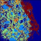
As an example, I’ve used the clustering function on a Landsat image of the Mississippi River. This 512 x 512 image has 7 channels. Working from the purely point-and-click Analysis interface on my 4 year old MacBook Pro laptop, this image can be clustered into 3 groups in 6.8 seconds. The result is shown at the far left. Clustering into 6 groups takes just a bit longer, 13.8 seconds. Results for the 6 cluster analysis are shown at the immediate left. This is actually a pretty good rendering of the different surface types in the image.

As another example, I’ve used the image clustering function on the SIMS image of a drug bead. This image is 256 x 256 and has 93 channels. For reference, the (contrast enhanced) PCA score image is shown at the far left. The drug bead coating is the bright green strip to the right of the image, while the active ingredient is hot pink. The same data clustered into 5 groups is shown to the immediate right. Computation time was 14.7 seconds. The same features are visible in the cluster image as the PCA, although the colors are swapped: the coating is dark brown and the active is bright blue.

Thanks, Jeremy!

BMW

Unscrambler X is out, and CAMO is touting the fact that it is 64-bit. We say, “Welcome to the party!” MATLAB has had 64-bit versions out since April, 2006. That means that users of our PLS_Toolbox and MIA_Toolbox software have enjoyed the ability to work with data sets larger than 2Gb for over 4 years now. Our stand-alone packages, Solo and Solo+MIA have been 64-bit since June, 2009.

And how much is Unscrambler X? They don’t post their prices like we do. So go ahead and get a quote on Unscrambler, and then compare. We think you’ll find our chemometric software solutions to be a much better value!

BMW

The age of Partial Least Squares (PLS) regression (as opposed to PLS path modeling) began with the SIAM publication of Svante Wold et. al. in 1984 [1]. Many of us learned PLS regression from the rather more accessible paper by Geladi and Kowalski from 1986 [2] which described the Nonlinear Iterative PArtial Least Squares (NIPALS) algorithm in detail.

For univariate y, the NIPALS algorithm is really more sequential than iterative. There is a specific sequence of fixed steps that are followed to find the weight vector w (generally normalized to unit length) for each PLS factor or Latent Variable (LV). Only in the case of multivariate Y is the algorithm really iterative, a sequence of steps is repeated until the solution for w for each LV converges.

Whether for univariate y or multivariate Y the calculations for each LV end with a deflation step. The X data is projected onto the weight vector w to get a score vector, t (t = Xw). X is then projected onto the score t to get a loading, p, (p = X’t/t’t). Finally, X is deflated by tp’ to form a new X, X_new with which to start the procedure again, X_new = X – tp’. A new weight vector w is calculated from the deflated X_new and the calculations continue.

So the somewhat odd thing about the weight vectors w derived from NIPALS is that each one applies to a different X, i.e. t_n+1 = X_nw_n+1. This is in contrast to Sijmen de Jong’s SIMPLS algorithm introduced in 1993 [3]. In SIMPLS a set of weights, sometimes referred to as R, is calculated, which operate on the original X data to calculate the scores. Thus, all the scores T can be calculated directly from X without deflation, T = XR. de Jong showed that it is easy to calculate the SIMPLS R from the NIPALS W and P, R = W(P’W)^-1. (Unfortunately, I have, as yet, been unable to come up with a simple expression for calculating the NIPALS W from the SIMPLS model parameters.)

So the question here is, “If you want to look at weights, which weights should you look at, W or R?” I’d argue that R is somewhat more intuitive as it applies to the original X data. Beyond that, if you are trying to standardize outputs of different software routines (which is actually how I got started on all this), it is a simple matter to always provide R. Fortunately, R and W are typically not that different, and in fact, they start out the same, w₁ = r₁, and they span the same subspace. Our decision here, based on relevance and standardization, is to present R weights as the default in future versions of PLS_Toolbox and Solo, regardless of which PLS algorithm is selected (NIPALS, SIMPLS or the new Direct Scores PLS).

A better question might be, “When investigating a PLS model, should I look at weights, R or W, or loadings P?” If your perspective is that the scores T are measures of some underlying “latent” phenomena, then you would choose to look at P, the degree to which these latent variables contribute to X. The weights W or R are merely regression coefficients that you use to estimate the scores T. From this viewpoint the real model is X = TP’ + E and y = Tb+ f.

If, on the other hand, you see PLS as simply a method for identifying a subspace within which to restrict, and therefore stabilize, the regression vector, then you would choose to look at the weights W or R. From this viewpoint the real model is Y = Xb + e, with b = W(P’W)^-1(T’T)^-1T’y = R(T’T)^-1T’y via the NIPALS and SIMPLS formulations respectively. The regression vector is a linear combination of the weights W or R and from this perspective the loadings P are really a red herring. In the NIPALS formulation they are a patch left over from the way the weights were derived from deflated X. And the loadings P aren’t even in the SIMPLS formulation.

So the bottom line here is that you’d look at loadings P if you are a fan of the latent variable perspective. If you’re a fan of the regression subspace perspective, then you’d look at weights, W or preferably R. I’m in the former camp, (for more reasons than just philosophical agreement with the LV model), as evidenced by my participation in S. Wold et. al., “The PLS model space revisited,” [4]. Your choice of perspective also impacts what residuals to monitor, etc., but I’ll save that for a later time.

BMW

[1] S. Wold, A. Ruhe, H. Wold, and W.J. Dunn III, “The Collinearity Problem in Linear
Regression. The Partial Least Square Approach to Generalized Inverses”, SIAM J. Sci.
Stat. Comput., Vol. 5, 735-743, 1984.

[2] P. Geladi and B.R. Kowalski, “PLS Tutorial,” Anal. Chim. Acta., 185(1), 1986.

[3] S. de Jong, “SIMPLS: an alternative approach to partial least squares regression,” Chemo. and Intell. Lab. Sys., Vol. 18, 251-263, 1993.

[4] S. Wold, M. Høy, H. Martens, J. Trygg, F. Westad, J. MacGregor and B.M. Wise, “The PLS model space revisited,” J. Chemometrics, pps 67-68, Vol. 23, No. 2, 2009.

NOTE: Current pricing can be found here.

That nip in the air in the morning means that back to school time has arrived. Kids of all ages are getting their supplies together, and so are their teachers.

If you are a student or instructor in a chemometrics or related class, we’ve got a deal for you! We’ll let you use demo versions of any of our data modeling software packages free-of-charge for six months. This includes our stand-alone products Solo and Solo+MIA, and our MATLAB toolboxes PLS_Toolbox, MIA_Toolbox and EMSC_Toolbox. All our demos are fully functional (no data size limitations), include all documentation and lots of example data sets.

To get started with the program, just write to me with information about the class our software will be used with (course title, instructor, start and end dates). If professors send their class list, we’ll set up accounts for all the students allowing them access to the extended demos. Alternately, students can set up their own accounts and let us know what class they are taking.

Many professors have gravitated towards using our Solo products. They don’t require MATLAB, so students can just download them and they’re ready to go. Solo and Solo+MIA work on Windows (32 and 64 bit) and Mac OS X.

BMW

The post I wrote on June 11, Referencing Software, resulted in a rather lengthy thread on ICS-L, the Chemometrics discussion list. Most discussants generally agreed that the software used to develop results for scientific papers should be referenced, including the software title, publisher, year and version number.

There were a few dissenters. Sergey Kucheryavski wrote:

…it makes sense only in two cases.
1. The software implements some unique, patented methods that are not available in any other programs.
2. There is a special agreement (caused by special price [e.g. PLS toolbox for 100 USD] or some other benefits) between user and a software company.

In a similar vein, Richard Brereton wrote:

If however software has been bought (often at considerable cost) I do not think this obliges the originator to cite it, there is no ethical requirement, unless the software was purchased at a specially low price…

I find this to be a rather interesting concept and wonder what would happen if we applied it to books as well. If I paid the $1595 for Comprehensive Chemometrics by Brown, Tauler and Walczak, do I not have to reference it? How about Brereton’s “Applied Chemometrics for Scientists?” Do I have to reference it because it’s only $110? Or do I have to reference it only if I get a discount off the list price? Clearly this is ridiculous.

Most of the respondents felt that it was important to reference software in order to assure reproducibility of the work. Philip Hopke wrote:

It seems to me that the fundamental issue is the ability of the reader of a paper to be able to fully replicate the work that has been published. If work is not replicable, then it is not science. The issue then is what is required to ensure repeatability of the … work being reported.

And I agree that this is the most important issue, but it is not the only issue. Bruce Kowalski wrote:

If ya’ll want a real debate start taking issue with publications that don’t mention the first paper in a research area. There has always been a correct way to use references. What went wrong???????

Referencing the first paper in a research area is all about giving credit where it’s due. It’s not about reproducibility, (which, as Cliff Spiegelman observed, is often better served by referencing later work, often done by someone other than the original author). Likewise, referencing software is also partly about giving credit where it’s due–recognizing the effort expended to produce a useful tool of scientific value.

BMW

Yesterday I picked up a newly-arrived journal and noted that the article highlighted on the front page looked quite interesting as we have been doing some related work. I eagerly turned to the article and found that the author had been using PLS-DA (Partial Least Squares Discriminant Analysis) and was, in fact, one of our PLS_Toolbox users. Imagine my disappointment when I could find no reference to our software in the article! The article had many references, with more than 50 journal articles cited and at least a half dozen equipment manufacturers named. But there was no mention of the software that was used to turn the measurements into the results that were presented.

I checked with the author of the article, and yes, our software was used to produce the results that were re-plotted in another application prior to publication. But exactly whose software was used is beside the point. The point is that software is a critical part of the experiment and, in order to ensure reproducibility, should be referenced.

Some might say that referencing the original work on the development of the particular analysis method implemented in the software should suffice, (though in this instance that wasn’t done either, the author referenced previous work of their own where they used PLS-DA). I’d argue that isn’t enough. The problem is that it typically takes a LOT of additional work to turn a method from an academic paper into a working program. There are often many special (sometimes schizophrenic) cases that must be handled properly to assure consistent results. Sometimes various meta-parameters must be optimized. Preprocessing can be critical. And then there is the whole interface which allows the user to interact with the data so that it can be effectively viewed, sorted and selected.

So why do I care? Obviously, there is the commercial aspect: having our software referenced is good advertising for us, and leads to more sales. But beyond that, (like many other publishers of scientific software, I’m sure), our software is probably our most significant work of scholarship. To not reference it is to not acknowledge the contributions we’ve made to the field.

So I’m calling on all authors to reference the software they use, and editors and reviewers to check that they do. Listing it in the references would be preferred. Software is, after all, a publication, with a title, version number (edition), publisher, and year of publication. Often, authors are also known, and can be listed. But one way or the other, software should be cited as it is critical to reproducibility and represents scholarly work upon which results depend. Referencing software upholds scientific and scholarly tradition and it is academically dishonest to not do so.

BMW