SEARCH
As part of our effort to make a future version of PLS_Toolbox compatible with the new MATLAB 2025a interface tools (and deprecation of Java) we surveyed our users to find out more about what they do and how they work. We got a nice response and some of the results were quite interesting, so I thought we’d share them here. We used Survey Monkey to conduct the survey so for the most part I just copied the figures from it.
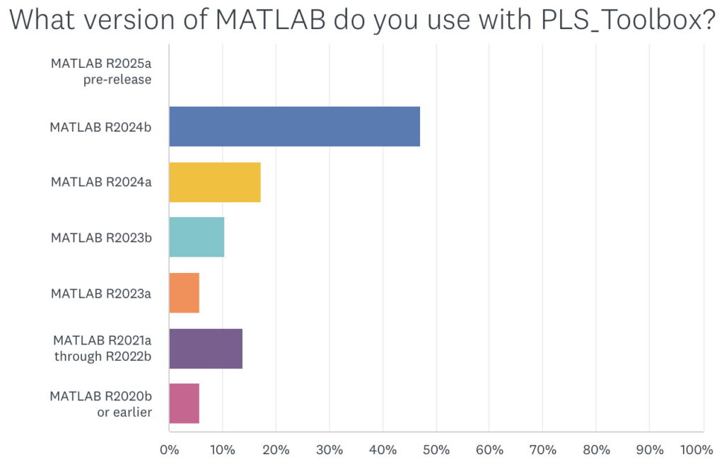
When asked what version of MATLAB was being used with PLS_Toolbox nearly 50% of our users responded with R2024b. This surprised me as I figured there would be a smaller percentage of users with the most current version of MATLAB. I’m reticent to update my MATLAB (and other software) versions unless I have a compelling reason to do so. My experience with R2024b is that it is an excellent release, (some are better than others), so that might be part of the reason. We also found that ~75% of users were on the current version of PLS_Toolbox, 9.5.
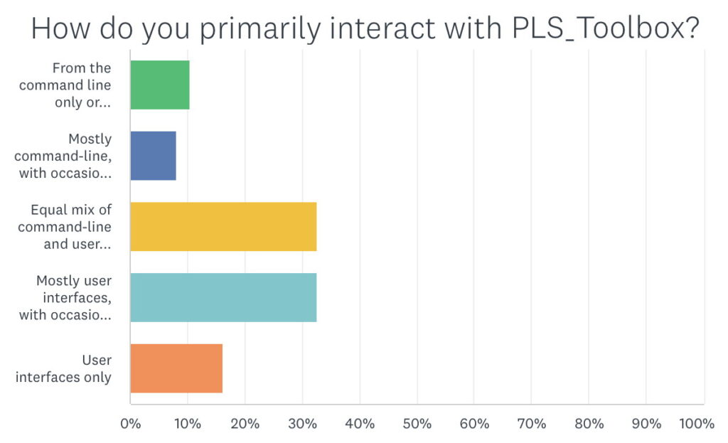
When asked how they primarily interacted with PLS_Toolbox about 75% answered with a mixture of use of the interfaces and use of the command line. The most frequent responses were an equal mix of both and mostly interfaces with occasional command line. I’m in this latter category myself. But this response really highlights one of the major strengths of PLS_Toolbox: you can use it either way. You can make models from the command line that are completely compatible with models generated by the interfaces, and vice-versa. How you work largely depends on the situation and personal preferences.
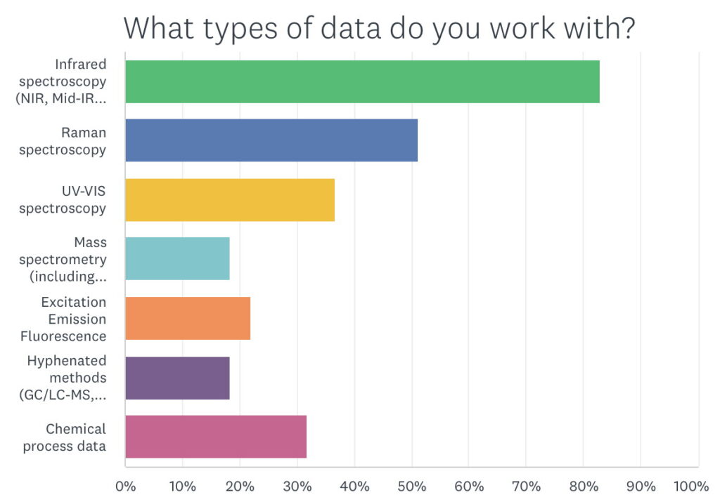
When asked about what types of data users were working with, it was no surprise that over 80% were working with NIR followed by 50% using Raman. Raman use has grown a lot in the last several years and we expect that trend to continue. UV-VIS was a larger group than I expected at a little over 35%. I was pleased that over 30% use it with chemical process data as that is how I got into this business to begin with. We were surprised to find that the “other” option produced quite a few instances of NMR use.
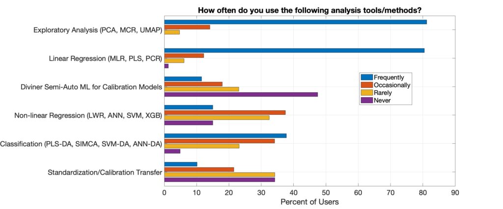
We asked our customers how frequently they used various analysis tools and methods. It was no surprise to us that over 80% did exploratory analysis, which includes PCA, frequently. Over 80% also use linear regression, which includes PLS, frequently. PCA and PLS are certainly the workhorses of chemical data science. About 70% of users accessed the classification methods in PLS_Toolbox at least occasionally while over 50% of them used the non-linear regression methods at least occasionally. Diviner, our new semi-automated machine learning tool for regression model development was used at least occasionally by about 30%. Given that Diviner is the newest major tool in PLS_Toolbox this seems like a good start and I expect that number to grow.
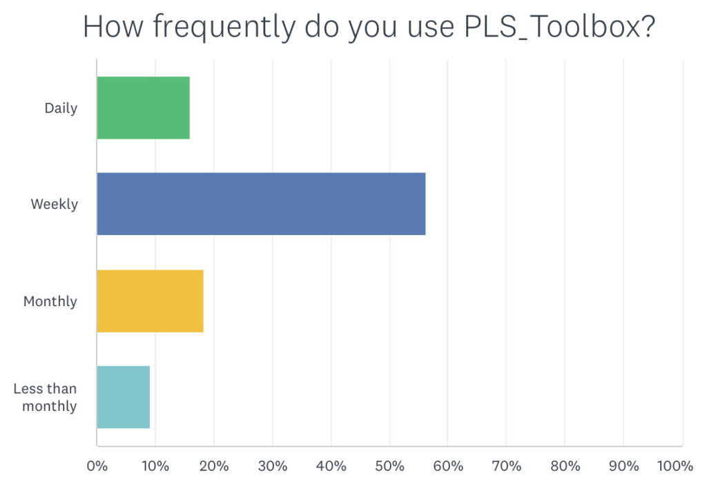
Over 70% of customers responding to the survey use PLS_Toolbox weekly or daily. Of course I expect that the heavier users were more likely to answer the survey, but still, that’s a lot. I only get a chance to use it weekly myself!
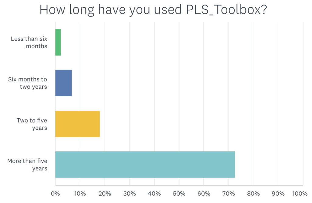
Many of our users have been with us for a long time. Over 70% responded that they’ve been using PLS_Toolbox for more than 5 years. When you combine that with the amount they use it above that accounts for a lot of use. This ultimately contributes to the reliability of PLS_Toolbox: issues get found and our development staff fixes them.
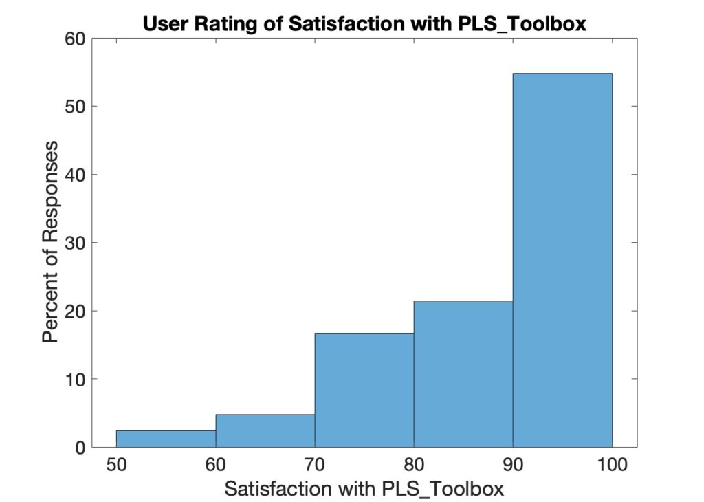
Finally, we asked users to rate their satisfaction with PLS_Toolbox on a scale from 1 to 100. A histogram of the responses is shown below. 55% of our customers gave PLS_Toolbox a rating of 90 or higher. The average was 86. Still room for improvement and of course we’re working on how to bring the bottom end of the scale up!
We of course asked users about what they find difficult and what they’d like us to add, etc., and got some good suggestions. So plenty to work on, as always! But I’ll leave my favorite comments here.
Love the product, creativity and quick support responsiveness!
Very complementary to my own MATLAB coding – often I jump back and forth. Nice PCA interface. I appreciate the missing data capabilities in a lot of the code.
I love Diviner. Please add preprocessing sets for the spectrosopic/chromatographic methods.
I have stuck with this product through the years as I trust the software, I find it very powerful (certainly better than anything my colleagues can do in free or shareware), and it is constantly changing and improving.
Thanks to all our users who completed the survey and provided this feedback!
BMW