 SEARCH
Category Archives: Chemometrics
Mediterranean Tour
Sep 17, 2010
I head off tomorrow morning (way too early!) on a “tour” of the Mediterranean. I’ll be attending The First African-European Conference on Chemometrics, aka Afrodata, in Rabat, Morocco. From there, I’ll go to CMA4CH–Application of MVA and Chemometrics to Cultural Heritage and Environment in Sicily. Then it’s on to Barcelona to teach Using the Advanced Features of PLS_Toolbox.
I’m looking forward to getting out of the office and spending some time with my chemometric colleagues. When I see something of chemometric interest during my travels, I’ll try to get it posted here. I hope to see many of you in the coming weeks!
BMW
One Last Time on Accuracy of PLS Algorithms
Sep 9, 2010
Scott Ramos of Infometrix wrote me last week and noted that he had followed the discussion on the accuracy of PLS algorithms. Given that they had done considerable work comparing their BIDIAG2 implementation with other PLS algorithms, he was “surprised” with my original post on the topic. He was kind enough to send me a MATLAB implementation of the PLS algorithms included in their product Pirouette for inclusion in my comparison.
Below you’ll find a figure that compares regression vectors from NIPALS, SIMPLS, DSPLS and the BIDIAG2 code provided by Scott. The figure was generated for a tall-skinny X-block (our “melter” data) and for a short-fat X-block (NIR of pseudo-gasoline mixture). Note that I used our SIMPLS and DSPLS that include re-orthogonalization, as that is now our default. While I haven’t totally grokked Scott’s code, I do see where it includes an explicit re-orthogonalization of the scores as well.

Note that all the algorithms are quite similar, with the biggest differences being less than one part in 1010. The BIDIAG2 code provided by Scott (hot pink with stars) is the closest to NIPALS for the tall skinny case, while being just a little more different than the other algorithms for the short fat case.
This has been an interesting exercise. I’m always surprised when I find there is still much to learn about something I’ve already been thinking about for 20+ years! It is certainly a good lesson in watching out for numerical accuracy issues, and in how accuracy can be improved with some rather simple modifications.
BMW
Coming in 6.0: Analysis Report Writer
Sep 4, 2010
Version 6.0 of PLS_Toolbox, Solo and Solo+MIA will be out this fall. There will be lots of new features, but right at the moment I’m having fun playing with one in particular: the Analysis Report Writer (ARW). The ARW makes documenting model development easy. Once you have a model developed, just make the plots you want to make, then select Tools/Report Writer in the Analysis window. From there you can select HTML, or if you are on a Windows PC, MS Word or MS Powerpoint for saving your report. The ARW then writes a document with all the details of your model, along with copies of all the figures you have open.
As an example, I’ve developed a (quick and dirty!) model using the tablet data from the IDRC shootout in 2002. The report shows the model details, including the preprocessing and wavelength selection, along with the plots I had up. This included the calibration curve, cross-validation plot, scores on first two PCs, and regression vector. But it could include any number and type of plots as desired by the user. Statistics on the prediction set are also included.
Look for Version 6.0 on our web site in October, or come visit us at FACSS, booth 48.
BMW
Re-orthogonalization of PLS Algorithms
Aug 23, 2010
Thanks to everybody that responded to the last post on Accuracy of PLS Algorithms. As I expected, it sparked some nice discussion on the chemometrics listserv (ICS-L)!
As part of this discussion, I got a nice note from Klaas Faber reminding me of the short communication he wrote with Joan Ferré, “On the numerical stability of two widely used PLS algorithms.” [1] The article compares the accuracy of PLS via NIPALS and SIMPLS as measured by the degree to which the scores vectors are orthogonal. It finds that SIMPLS is not as accurate as NIPALS, and suggests adding a re-orthogonalization step to the algorithms.
I added re-orthogonalization to the code for SIMPLS, DSPLS, and Bidiag2 and ran the tests again. The results are shown below. Adding this to Bidiag2 produces the most dramatic effect (compare to figure in previous post), and improvement is seen with SIMPLS as well. Now all of the algorithms stay within ~1 part in 1012 of each other through all 20 LVs of the example problem. Reconstruction of X from the scores and loadings (or weights, as the case may be!) was improved as well. NIPALS, SIMPLS and DSPLS all reconstruct X to within 3e-16, while Biadiag2 comes in at 6e-13.

The simple fix of re-orthogonalization makes Bidiag2 behave acceptably. I certainly would not use this algorithm without it! Whether to add it to SIMPLS is a little more debatable. We ran some tests on typical regression problems and found that the difference on predictions with and without it was typically around 1 part in 108 for models with the correct number of LVs. In other words, if you round your predictions to 7 significant digits or less, you’d never see the difference!
That said, we ran a few tests to determine the effect on computation time of adding the re-orthogonalization step to SIMPLS. For the most part, the effect was negligible, less than 5% additional computation time for the vast majority of problem sizes and at worst a ~20% increase. Based on this, we plan to include re-orthogonalization in our SIMPLS code in the next major release of PLS_Toolbox and Solo, Version 6.0, which will be out this fall. We’ll put it in the option to turn it off, if desired.
BMW
[1] N.M. Faber and J. Ferré, “On the numerical stability of two widely used PLS algorithms,” J. Chemometrics, 22, pps 101-105, 2008.
Accuracy of PLS Algorithms
Aug 13, 2010
In 2009 Martin Andersson published “A comparison of nine PLS1 algorithms” in Journal of Chemometrics[1]. This was a very nice piece of work and of particular interest to me as I have worked on PLS algorithms myself [2,3] and we include two algorithms (NIPALS and SIMPLS) in PLS_Toolbox and Solo. Andersson compared regression vectors calculated via nine algorithms using 16 decimal digits (aka double precision) in MATLAB to “precise” regression vectors calculated using 1000 decimal digits. He found that several algorithms, including the popular Bidiag2 algorithm (developed by Golub and Kahan [4] and adapted to PLS by Manne [5]), deviated substantially from the vectors calculated in high precision. He also found that NIPALS was among the most stable of algorithms, and while somewhat less accurate, SIMPLS was very fast.
Andersson also developed a new PLS algorithm, Direct Scores PLS (DSPLS), which was designed to be accurate and fast. I coded it up, adapted it to multivariate Y, and it is now an option in PLS_Toolbox and Solo. In the process of doing this I repeated some of Andersson’s experiments, and looked at how the regression vectors calculated by NIPALS, SIMPLS, DSPLS and Bidiag2 varied.
The figure below shows the difference between various regression vectors as a function of Latent Variable (LV) number for Melter data set, where X is 300 x 20. The plotted values are the norm of the difference divided by the norm the first regression vector. The lowest line on the plot (green with pluses) is the difference between the NIPALS and DSPLS regression vectors. These are the two methods that are in the best agreement. DSPLS and NIPALS stay within 1 part in 1012 out through the maximum number of LVs (20).

The next line up on the plot (red line and circles with blue stars) is actually two lines, the difference between SIMPLS and both NIPALS and DSPLS. These lie on top of each other because NIPALS and DSPLS are so similar to each other. SIMPLS stays within one part in 1010 through 10 LVs (maximum LVs of interest in this data) and degrades to one part in ~107.
The highest line on the plot (pink with stars) is the difference between NIPALS and Bidiag2. Note that by 9 LVs this difference has increased to 1 part in 100, which is to say that the regression vector calculated by Bidiag2 has no resemblance to the regression vector calculated by the other methods!
I programmed my version of Bidiag2 following the development in Bro and Eldén [6]. Perhaps there exist more accurate implementations of Bidiag2, but my results resemble those of Andersson quite closely. You can download my bidiag.m file, along with the code that generates this figure, check_PLS_reg_accuracy.m. This would allow you to reproduce this work in MATLAB with a copy of PLS_Toolbox (a demo would work). I’d be happy to incorporate an improved version of Bidiag in this analysis, so if you have one, send it to me.
BMW
[1] Martin Andersson, “A comparison of nine PLS1 algorithms,” J. Chemometrics, 23(10), pps 518-529, 2009.
[2] B.M. Wise and N.L. Ricker, “Identification of Finite Impulse Response Models with Continuum Regression,” J. Chemometrics, 7(1), pps 1-14, 1993.
[3] S. de Jong, B. M. Wise and N. L. Ricker, “Canonical Partial Least Squares and Continuum Power Regression,” J. Chemometrics, 15(2), pps 85-100, 2001.
[4] G.H. Golub and W. Kahan, “Calculating the singular values and pseudo-inverse of a matrix,” SIAM J. Numer. Anal., 2, pps 205-224, 1965.
[5] R. Manne, “Analysis of two Partial-Least-Squares algorithms for multivariate calibration,” Chemom. Intell. Lab. Syst., 2, pps 187–197, 1987.
[6] R. Bro and L. Eldén, “PLS Works,” J. Chemometrics, 23(1-2), pps 69-71, 2009.
Clustering in Images
Aug 6, 2010
It is probably an understatement to say that here are many methods for cluster analysis. However, most clustering methods don’t work well for large data sets. This is because they require computation of the matrix that defines the distance between all the samples. If you have n samples, then this matrix is n x n. That’s not a problem if n = 100, or even 1000. But in multivariate images, each pixel is a sample. So a 512 x 512 image would have a full distance matrix that is 262,144 x 262,144. This matrix would have 68 billion elements and take 524G of storage space in double precision. Obviously, that would be a problem on most computers!
In MIA_Toolbox and Solo+MIA there is a function, developed by our Jeremy Shaver, which works quite quickly on images (see cluster_img.m). The trick is that it chooses some unique seed points for the clusters by finding the points on the outside of the data set (see distslct_img.m), and then just projects the remaining data onto those points (normalized to unit length) to determine the distances. A robustness check is performed to eliminate outlier seed points that result in very small clusters. Seed points can then be replaced with the mean of the groups, and the process repeated. This generally converges quite quickly to a result very similar to knn clustering, which could not be done in a reasonable amount of time for large images.

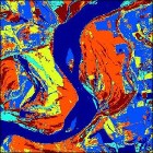 As an example, I’ve used the clustering function on a Landsat image of the Mississippi River. This 512 x 512 image has 7 channels. Working from the purely point-and-click Analysis interface on my 4 year old MacBook Pro laptop, this image can be clustered into 3 groups in 6.8 seconds. The result is shown at the far left. Clustering into 6 groups takes just a bit longer, 13.8 seconds. Results for the 6 cluster analysis are shown at the immediate left. This is actually a pretty good rendering of the different surface types in the image.
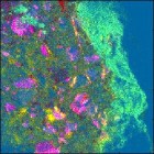
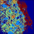 As another example, I’ve used the image clustering function on the SIMS image of a drug bead. This image is 256 x 256 and has 93 channels. For reference, the (contrast enhanced) PCA score image is shown at the far left. The drug bead coating is the bright green strip to the right of the image, while the active ingredient is hot pink. The same data clustered into 5 groups is shown to the immediate right. Computation time was 14.7 seconds. The same features are visible in the cluster image as the PCA, although the colors are swapped: the coating is dark brown and the active is bright blue.
Thanks, Jeremy!
BMW
Pseudoinverses, Rank and Significance
Jun 1, 2010
The first day of Eigenvector University 2010 started with a class on Linear Algebra, the “language of chemometrics.” The best question of the day occurred near the end of the course as we were talking about pseudoinverses. We were doing an example with a small data set, shown below, which demonstrates the problem of numerical instability in regression.
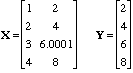
If you regress Y on X you get regression coefficients of b = [2 0]. On the other hand, if you change the 3rd element of Y to 6.0001, you get b = [3.71 -0.86]. And if you you change this element to 5.9999, then b = [0.29 0.86]. So a change of 1 part in 50,000 in Y changes the answer for b completely.
The problem, of course, is that X is nearly rank deficient. If it weren’t for the 0.0001 added to the 8 in the (4,2) element X would be rank 1. If you use the Singular Value Decomposition (SVD) to do a rank 1 approximation of X and use that for the pseudoinverse, the problem is stabilized. In MATLAB-ese, this is [U,S,V] = svd(X), then Xinv = V(:,1)*inv(S(1,1))*U(:,1)’, and b = Xinv*Y = [0.40 0.80]. If you choose 5.9999, 6.0000 or 6.0001 for the 3rd element of Y, the answer for b stays the same to within 0.00001.
Then the question came: “Why don’t you get the stable solution when you use the pseudoinverse function, pinv, in MATLAB?” The answer is that, to MATLAB, X is not rank 1, it is rank 2. The singular values of X are 12.2 and 3.06e-5. MATLAB would consider a singular value zero if it was less than s = max(size(X))*norm(X)*eps, where eps is the machine precision. In this instance, s = 1.08e-14, and the smaller singular value of X is larger than this by about 9 orders of magnitude.
But just because it is significant with respect to machine precision doesn’t mean that is significant with respect to the precision of the measurements. If X was measured values, and it was known that they could only be reliably measured to 0.001, then clearly the rank 1 approximation of X should be used for this problem. In MATLAB, you can specify the tolerance of the pinv function. So if you use, for instance, Xinv = pinv(X,1e-4), then you get the same stable solution we did when we used the rank 1 approximation explicitly.
Thanks for the good question!
BMW
Eigenvector University 2010 Best Posters
May 26, 2010
The EigenU 2010 Poster Session was held Tuesday evening, May 18. This year 7 users contributed posters for the contest, and the Eigenvectorians chipped in another 5, so there was plenty to discuss. We all enjoyed beer, wine and hors d’oeuvres as we discussed the finer points of aligning chromatograms and calculating PARAFAC models, among other things!
This year’s posters were judged by Bruce Kowalski, guest instructor at this year’s EigenU, and Brian Rohrback, President of Infometrix. Bruce and Brian carefully reviewed the submitted posters (not counting the ones from the Eigenvectorians, of course). Thanks to the judges, especially Brian, who stopped by just for this event!

Barry Wise, Jamin Hoggard, Bruce Kowalski, Cagri Ozcaglar and Brian Rohrback
The winners, pictured above, were Cagri Ozcaglar of Rensselaer Polytechnic Institute for Examining Sublineage Structure of Mycobacterium Tuberculosis Complex Strains with Multiway Modeling, and Jamin Hoggard of the University of Washington for Extended Nontarget PARAFAC Applications to GC×GC–TOF-MS Data. Jamin and Cagri accepted iPod nanos with the inscription Eigenvector University 2010 Best Poster for their efforts.
Congratulations, Cagri and Jamin!
BMW
Biggest Chemometrics Learning Event Ever?
May 26, 2010
Eigenvector University 2010 finished up on Friday afternoon, May 21. What a week! Six days, 17 courses, 10 instructors and 45 students. I’d venture a guess that this was the biggest chemometrics learning event ever. If more chemometrics students and instructors have been put together for more hours than in Seattle last week, I’m not aware of it.
Thanks to all that came for making it such a great event. It was a very accomplished audience, and the discussions were great, both in class and over beers. The group fielded lots of good questions, observations and related much useful experience.
We’re already looking forward to doing it next year and have been busy this week incorporating student feedback into our courses and software. The Sixth Edition of EigenU is tentatively scheduled for May 15-20, 2011. See you there!
BMW
Robust Methods
May 12, 2010
This year we are presenting “Introduction to Robust Methods” at Eigenvector University. I’ve been working madly preparing a set of course notes. And I must say that it has been pretty interesting. I’ve had a chance to try the robust versions of PCA, PCR and PLS on many of the data sets we’ve used for teaching and demoing software, and I’ve been generally pleased with the results. Upon review of my course notes, our Donal O’Sullivan asked why we don’t use the robust versions of these methods all the time. I think that is a legitimate question!
In a nutshell, robust methods work by finding the subset of samples in the data that are most consistent. Typically this involves use of the Minimum Covariance Determinant (MCD) method, which finds the samples that have a covariance with the smallest determinant, which is a measure of the volume occupied by the data. The user specifies the fraction, h, to include, and the algorithm searches out the optimal set. The parameter h is between 0.5 and 1, and a good general default is 0.75. With h = 0.75 the model can resist up to 25% arbitrarily bad samples without going completely astray. After finding the h subset, the methods then look to see what remaining samples fall within the statistical bounds of the model and re-include them. Any remaining samples are considered outliers.
The main advantage of robust methods is that they automate the process of finding outliers. This is especially convenient when the data sets have many samples and a substantial fraction of bad data. How many times have you removed an obvious outlier from a data set only to find another outlier that wasn’t obvious until the first one is gone? This problem, known as masking, is virtually eliminated with robust methods. Swamping, when normal samples appear as outliers due to the confidence limits being stretched by the true outliers, is also mitigated.
So am I ready to set my default algorithm preferences to “robust?” Well, not quite. There is some chance that useful samples, sometimes required for building the model over a wide range of the data, will be thrown out. But I think I’ll at least review the robust results now each time I make a model on any medium or large data set, and consider why the robust method identifies them as outliers.
FYI, for those of you using PLS_Toolbox or Solo, you can access the robust option in PCA, PCR and PLS from the analysis window by choosing Edit/Options/Method Options.
Finally, I should note that the robust methods in our products are there due to a collaboration with Mia Hubert and her Robust Statistics Group at Katholieke Universiteit Leuven, and in particular, Sabine Verboven. They have been involved with the development of LIBRA, A MATLAB LIBrary for Robust Analysis. Our products rely on LIBRA for the robust “engines.” Sabine spent considerable time with us helping us integrate LIBRA into our software. Many thanks for that!
BMW
Welcome to the 64-bit party!
May 3, 2010
Unscrambler X is out, and CAMO is touting the fact that it is 64-bit. We say, “Welcome to the party!” MATLAB has had 64-bit versions out since April, 2006. That means that users of our PLS_Toolbox and MIA_Toolbox software have enjoyed the ability to work with data sets larger than 2Gb for over 4 years now. Our stand-alone packages, Solo and Solo+MIA have been 64-bit since June, 2009.
And how much is Unscrambler X? They don’t post their prices like we do. So go ahead and get a quote on Unscrambler, and then compare. We think you’ll find our chemometric software solutions to be a much better value!
BMW
Best Poster iPods Ordered
Apr 28, 2010
As in past years, this year’s Eigenvector University includes a poster session where users of MATLAB, PLS_Toolbox and Solo can showcase their work in the field of chemometrics. It is also a chance to discuss unsolved problems and future directions, over a beer, no less.
This year’s crop of posters will be judged by Bruce Kowalski, co-founder of the field of chemometrics. For their efforts, the top two poster presenters will receive Apple iPod nanos! This year I’ve ordered the 16GB models that record and display video and include an FM tuner with Live Pause. These are spiffy, for sure. We’ll have one in blue (just like the EVRI logo!) and one in orange (our new highlight color, new website coming soon!). Both are engraved “Eigenvector University 2010, Best Poster.”
There is still time to enter the poster contest. Just send your abstract, describing your chemometric achievements and how you used MATLAB and/or our products, to me, bmw@eigenvector.com. Then be ready to present your poster at the Washington Athletic Club in downtown Seattle, at 5:30pm on Tuesday, May 18. The poster session is free, no need to register for EigenU classes.
You could win!
BMW
EigenU 2010 on-track to be biggest ever
Apr 18, 2010
The Fifth Edition of Eigenvector University is set for May 16-21, 2010. Once again we’ll be at the beautiful Washington Athletic Club in Seattle. This year we’ll be joined by Bruce Kowalski, co-founder (with Svante Wold) of the field of Chemometrics. Rasmus Bro will also be there, along with the entire Eigenvector staff.
Registrations are on-track to make this the biggest EigenU ever. All of the 17 classes on the schedule are a go! We’re also looking forward to Tuesday evening’s Poster Session (with iPod nano prizes), Wednesday evening’s PowerUser Tips & Tricks session, and Thursday evening’s Workshop Dinner. It is going to be a busy week!
BMW
Chemometric “how to” videos on-line
Nov 12, 2009
If a picture is worth a thousand words, what’s a video worth?
Here at EVRI we’ve started developing a series of short videos that show “how to” do various chemometric tasks with our software packages, including our new PLS_Toolbox 5.5 and Solo 5.5. Some of the presentations are pretty short and specific, but others are a little longer (10-15 minutes) and are a blend of teaching a bit about the method being used while showing how to do it in the software.
An example of the latter is “PCA on Wine Data” which shows how to build a Principal Components Analysis model on a small data set concerning the drinking habits, health and longevity of the population of 10 countries. Another movie, “PLS on Tablet Data” demonstrates building a Partial Least Squares calibration for a NIR spectrometer to predict assay values in pharmaceutical tablets.
While I was at it, I just couldn’t help producing a narrated version of our “Eigenvector Company Profile.”
We plan to have many more of these instructional videos that cover aspects of chemometrics and our software from basic to advanced. We hope you find each of them worth at least 1000 words!
BMW
Carl Duchesne Wins Best Poster at MIA Workshop
Oct 27, 2009
The International Workshop on Multivariate Image Analysis was held September 28-29 in Valencia, Spain. We weren’t able to make it, but we were happy to sponsor the Best Poster prize, which was won by Carl Duchesne. Carl is an Assistant Professor at Université Laval, in Sainte-Foy, Quebec, CA, where he works with the Laboratoire d’observation et d’optimisation des procédés (LOOP).
With co-authors Ryan Gosselin and Denis Rodrigue, Prof. Duchesne presented “Hyperspectral Image Analysis and Applications in Polymer Processing.” The poster describes how a spectral imaging system combined with texture analysis can be used with multivariate models to predict the thermo-mechanical properties of polymers during their manufacture. The system can also be used to detect abnormal processing conditions, what we would call Multivariate Statistical Process Control (MSPC).
For his efforts Carl received a copy of our Solo+MIA software, which is our stand-alone version of PLS_Toolbox + MIA_Toolbox. We trust that Carl and his group at Laval will find it useful in their future MIA endeavors. Congratulations Carl!
BMW
FACSS 2009 Wrap-up
Oct 27, 2009
Once again, the Federation of Analytical and Spectroscopy Societies conference, FACSS 2009, has drawn to a successful close. As usual, Eigenvector was there with a booth in the trade show, short courses, and talks.
We were very pleased at the popularity of our Chemometrics without Equations (CWE) and Advanced Chemometrics without Equations (ACWE) courses this year. CWE, led by our Bob Roginski, was at capacity with 20 students. I headed up ACWE, which was nearly full with 17. The courses were hands-on and gave the students a chance to test out the newest versions of our software, the soon to be released PLS_Toolbox 5.5 and MIA_Toolbox 2.0. Thanks to all who attended!
Our Jeremy Shaver gave two talks in the technical sessions. The first, “Soft versus Hard Orthogonalization Filters in Classification Modeling” provided an overview of numerous methods for developing filters. The bottom line is that all of the methods considered, including Orthogonal Signal Correction (OSC), Orthogonal PLS (O-PLS), Modified OSC (M-OSC), External Parameter Orthogonalization (EPO), and Generalized Least Squares weighting (GLS) perform very similarly.
Jeremy also presented “Analyzing and Visualizing Large Raman Images,” which was a joint work with Eunah Lee and Andrew Whitley of HORIBA Jobin Yvon, plus our own R. Scott Koch. This talk presented a method for doing PCA on multivariate images for situations where the entire data set cannot fit into computer memory. “Sequential PCA with updating” was shown to produce a very close approximation to conventional PCA. This is one potential strategy for dealing with the huge imaging data sets that are becoming increasingly common.
We’d like to thank the organizers of FACSS for another great meeting. We’re looking forward to the next one in Raleigh, NC, next year!
BMW
Continuum Regression illustrates differences between PCR, PLS and MLR
Sep 18, 2009
There has been a discussion this week on the International Chemometrics Society List (ICS-L) involving differences between Principal Components Regression (PCR), Partial Least Squares (PLS) regression and Multiple Linear Regression (MLR). This has brought up the subject of Continuum Regression (CR), which is one of my favorite topics!
I got into CR when I was working on my dissertation as it was a way to unify PCR, PLS and MLR so that their similarities and differences might be more thoroughly understood. CR is a continuously adjustable regression technique that encompasses PLS and includes PCR and MLR as opposite ends of the continuum. In CR the regression vector is a function the continuum parameter and of how many Latent Variables (LVs) are included in the model.
The continuum regression prediction error surface has been the logo for PLS_Toolbox since version 1.5 (1995). We use it in our courses because it graphically illustrates several important aspects of these regression methods. The CR prediction error surface is shown below
The CR prediction error surface illustrates the following points:
1) Models with enough LVs converge to the MLR solution. There is a region of models near the MLR side with many LVs that all have the same prediction error, this is the flat green surface on the right. These models have enough LVs in them so they have all converged to the MLR solution.
2) Models with too few or irrelevant factors have large prediction error. The large errors on the left are from models with few factors nearer the PCR side. These models don’t have enough factors (or at least enough of the right factors) in them to be very predictive. Note also the local maximum along the PCR edge at 4 LVs. This illustrates how often some of the PCR factors are not relevant for prediction (no surprise, as they are determined only by the amount of predictor X variance captured) so they lead to larger errors when included.
3) PLS is much less likely to have irrelevant factors than PCR. The prediction error curve for PLS doesn’t show these local maxima because of the way the factors are determined using information from the predicted variable y, i.e. they are based on covariance.
4) PLS models have fewer factors than PCR models. The bottom of the trough, aka the “valley of best models” runs at an angle through the surface, showing that PLS models generally hit their minimum prediction error with fewer factors than PCR models. Of course, near the MLR extreme, they hit the minimum with just 1 factor!
5) PLS models are not more parsimonious than PCR models. The angle of the valley of best models through the surface illustrates that PLS models are not really more parsimonious just because they have few factors. They are, in fact, “trying harder” to be correlated with the predicted variable y and (as Hilko van der Voet has shown) are consuming more degrees of freedom in doing so. If PLS was more parsimonious than PCR just based on the number of factors, then the 1 factor CR model near MLR would be even better, and we know it’s not!
CR has been in PLS_Toolbox since the first versions. It is not a terribly practical technique, however, as it is difficult to choose the “best” place to be in the continuum. But it really illustrates the differences between the methods nicely. If you have an interest in CR, I suggest you see:
B.M. Wise and N.L. Ricker, “Identification of Finite Impulse Response Models with Continuum Regression,” Journal of Chemometrics, 7(1), pps. 1-14, 1993.
and
S. de Jong, B. M. Wise and N. L. Ricker, “Canonical Partial Least Squares and Continuum Power Regression,” Journal of Chemometrics, 15(2), pps 85-100, 2001.
BMW
Chemometrics at SIMS XVII
Sep 17, 2009
The the 17th International Conference on Secondary Ion Mass Spectrometry, SIMS XVII, is being held this week in Toronto, CA. I am here with our Willem Windig. I’ve had an interest in SIMS for about a dozen years now, after being introduced to it by Anna Belu. Anna invited me to do a workshop on chemometrics in SIMS, gave me some data sets to work with, and off I went. SIMS was especially interesting to me because it provides very rich data sets, and is also often done over surfaces, producing what we refer to as multivariate images.
The use of chemometric techniques in SIMS has expanded considerably since I first got involved. The primary tool is still Principal Components Analysis (PCA), though there are certainly applications of other methods, including Maximal Autocorrelation Factors (MAF). However, I still see lots of examples where authors present 10, 20 or even 30 (!) images at different masses that are obviously highly correlated. These images could be replaced with one or two scores images and corresponding loadings plots: there would be less to look at, the images would be clearer due to the noise reduction aspects of PCA, and more might be learned about the chemistry from the loadings. So we still have a way to go before we reach everybody!
Over the years I’ve learned quite a bit about the non-idealities in SIMS. It certainly isn’t like like NIR spectra that follow Beer’s Law and have very high signal-to-noise! But I’ve gotten an additional appreciation for some of the issues from some of the talks here. There are plenty of “problems” such as detector dead time, low ion count statistics, effects due to topography, etc., which must be considered while doing an analysis.
I’ve been known to say that the secret to EVRI is data preprocessing, i.e. what you do the data before it hits the analysis method, e.g. PCA or PLS. That is certainly true with SIMS, and it’s nice to see that this is well appreciated among this group. The challenge for us as software developers will be to integrate these “correction” methods into our packages in a way that makes using them convenient.
I think that SIMS is ripe for more applications of Multivariate Curve Resolution (MCR), and in fact we focused quite a bit on that in our course here, Chemometrics in SIMS. With proper preprocessing, many applications of curve resolution should be possible. The more chemically meaningful results should be a hit with this audience, I would think.
I hope to see more MCR by the time of the SIMS XVIII, which will be held in Riva del Garda, ITALY, September 18-23, 2011. I plan to keep working in this area, if only so I can go to that! Hope to see you there.
BMW
Different kinds of PLS weights, loadings, and what to look at?
Sep 12, 2009
The age of Partial Least Squares (PLS) regression (as opposed to PLS path modeling) began with the SIAM publication of Svante Wold et. al. in 1984 [1]. Many of us learned PLS regression from the rather more accessible paper by Geladi and Kowalski from 1986 [2] which described the Nonlinear Iterative PArtial Least Squares (NIPALS) algorithm in detail.
For univariate y, the NIPALS algorithm is really more sequential than iterative. There is a specific sequence of fixed steps that are followed to find the weight vector w (generally normalized to unit length) for each PLS factor or Latent Variable (LV). Only in the case of multivariate Y is the algorithm really iterative, a sequence of steps is repeated until the solution for w for each LV converges.
Whether for univariate y or multivariate Y the calculations for each LV end with a deflation step. The X data is projected onto the weight vector w to get a score vector, t (t = Xw). X is then projected onto the score t to get a loading, p, (p = X’t/t’t). Finally, X is deflated by tp’ to form a new X, Xnew with which to start the procedure again, Xnew = X – tp’. A new weight vector w is calculated from the deflated Xnew and the calculations continue.
So the somewhat odd thing about the weight vectors w derived from NIPALS is that each one applies to a different X, i.e. tn+1 = Xnwn+1. This is in contrast to Sijmen de Jong’s SIMPLS algorithm introduced in 1993 [3]. In SIMPLS a set of weights, sometimes referred to as R, is calculated, which operate on the original X data to calculate the scores. Thus, all the scores T can be calculated directly from X without deflation, T = XR. de Jong showed that it is easy to calculate the SIMPLS R from the NIPALS W and P, R = W(P’W)-1. (Unfortunately, I have, as yet, been unable to come up with a simple expression for calculating the NIPALS W from the SIMPLS model parameters.)
So the question here is, “If you want to look at weights, which weights should you look at, W or R?” I’d argue that R is somewhat more intuitive as it applies to the original X data. Beyond that, if you are trying to standardize outputs of different software routines (which is actually how I got started on all this), it is a simple matter to always provide R. Fortunately, R and W are typically not that different, and in fact, they start out the same, w1 = r1, and they span the same subspace. Our decision here, based on relevance and standardization, is to present R weights as the default in future versions of PLS_Toolbox and Solo, regardless of which PLS algorithm is selected (NIPALS, SIMPLS or the new Direct Scores PLS).
A better question might be, “When investigating a PLS model, should I look at weights, R or W, or loadings P?” If your perspective is that the scores T are measures of some underlying “latent” phenomena, then you would choose to look at P, the degree to which these latent variables contribute to X. The weights W or R are merely regression coefficients that you use to estimate the scores T. From this viewpoint the real model is X = TP’ + E and y = Tb+ f.
If, on the other hand, you see PLS as simply a method for identifying a subspace within which to restrict, and therefore stabilize, the regression vector, then you would choose to look at the weights W or R. From this viewpoint the real model is Y = Xb + e, with b = W(P’W)-1(T’T)-1T’y = R(T’T)-1T’y via the NIPALS and SIMPLS formulations respectively. The regression vector is a linear combination of the weights W or R and from this perspective the loadings P are really a red herring. In the NIPALS formulation they are a patch left over from the way the weights were derived from deflated X. And the loadings P aren’t even in the SIMPLS formulation.
So the bottom line here is that you’d look at loadings P if you are a fan of the latent variable perspective. If you’re a fan of the regression subspace perspective, then you’d look at weights, W or preferably R. I’m in the former camp, (for more reasons than just philosophical agreement with the LV model), as evidenced by my participation in S. Wold et. al., “The PLS model space revisited,” [4]. Your choice of perspective also impacts what residuals to monitor, etc., but I’ll save that for a later time.
BMW
[1] S. Wold, A. Ruhe, H. Wold, and W.J. Dunn III, “The Collinearity Problem in Linear
Regression. The Partial Least Square Approach to Generalized Inverses”, SIAM J. Sci.
Stat. Comput., Vol. 5, 735-743, 1984.
[2] P. Geladi and B.R. Kowalski, “PLS Tutorial,” Anal. Chim. Acta., 185(1), 1986.
[3] S. de Jong, “SIMPLS: an alternative approach to partial least squares regression,” Chemo. and Intell. Lab. Sys., Vol. 18, 251-263, 1993.
[4] S. Wold, M. Høy, H. Martens, J. Trygg, F. Westad, J. MacGregor and B.M. Wise, “The PLS model space revisited,” J. Chemometrics, pps 67-68, Vol. 23, No. 2, 2009.
Back to School Deals for Chemometrics Novices
Aug 26, 2009
NOTE: Current pricing can be found here.
That nip in the air in the morning means that back to school time has arrived. Kids of all ages are getting their supplies together, and so are their teachers.
If you are a student or instructor in a chemometrics or related class, we’ve got a deal for you! We’ll let you use demo versions of any of our data modeling software packages free-of-charge for six months. This includes our stand-alone products Solo and Solo+MIA, and our MATLAB toolboxes PLS_Toolbox, MIA_Toolbox and EMSC_Toolbox. All our demos are fully functional (no data size limitations), include all documentation and lots of example data sets.
To get started with the program, just write to me with information about the class our software will be used with (course title, instructor, start and end dates). If professors send their class list, we’ll set up accounts for all the students allowing them access to the extended demos. Alternately, students can set up their own accounts and let us know what class they are taking.
Many professors have gravitated towards using our Solo products. They don’t require MATLAB, so students can just download them and they’re ready to go. Solo and Solo+MIA work on Windows (32 and 64 bit) and Mac OS X.
BMW