Clustering in Images

It is probably an understatement to say that here are many methods for cluster analysis. However, most clustering methods don’t work well for large data sets. This is because they require computation of the matrix that defines the distance between all the samples. If you have n samples, then this matrix is n x n. That’s not a problem if n = 100, or even 1000. But in multivariate images, each pixel is a sample. So a 512 x 512 image would have a full distance matrix that is 262,144 x 262,144. This matrix would have 68 billion elements and take 524G of storage space in double precision. Obviously, that would be a problem on most computers!

In MIA_Toolbox and Solo+MIA there is a function, developed by our Jeremy Shaver, which works quite quickly on images (see cluster_img.m). The trick is that it chooses some unique seed points for the clusters by finding the points on the outside of the data set (see distslct_img.m), and then just projects the remaining data onto those points (normalized to unit length) to determine the distances. A robustness check is performed to eliminate outlier seed points that result in very small clusters. Seed points can then be replaced with the mean of the groups, and the process repeated. This generally converges quite quickly to a result very similar to knn clustering, which could not be done in a reasonable amount of time for large images.

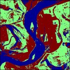
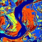As an example, I’ve used the clustering function on a Landsat image of the Mississippi River. This 512 x 512 image has 7 channels. Working from the purely point-and-click Analysis interface on my 4 year old MacBook Pro laptop, this image can be clustered into 3 groups in 6.8 seconds. The result is shown at the far left. Clustering into 6 groups takes just a bit longer, 13.8 seconds. Results for the 6 cluster analysis are shown at the immediate left. This is actually a pretty good rendering of the different surface types in the image.

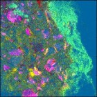
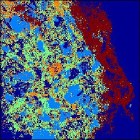As another example, I’ve used the image clustering function on the SIMS image of a drug bead. This image is 256 x 256 and has 93 channels. For reference, the (contrast enhanced) PCA score image is shown at the far left. The drug bead coating is the bright green strip to the right of the image, while the active ingredient is hot pink. The same data clustered into 5 groups is shown to the immediate right. Computation time was 14.7 seconds. The same features are visible in the cluster image as the PCA, although the colors are swapped: the coating is dark brown and the active is bright blue.

Thanks, Jeremy!

BMW