Classical Least Squares (CLS) with Nonlinear Spectra

In the last several years we’ve seen a resurgence of interest in Classical Least Squares (CLS) modeling. To address that our Neal Gallagher is developing a course on CLS Methods for the next EigenU. Our interest also stems from the fact that we’ve worked on a number of consulting projects where CLS models are appropriate for calibrating spectroscopic systems. As you might expect, these systems are relatively simple mixtures in gas or liquid phase. Recall the CLS model is

X = CS‘ + E

where X is the measured spectra, C is the matrix of concentrations, S is the pure component spectra and E is noise.

Complicating matters a bit, several of the systems we’ve worked with exhibit significant nonlinearities due to high absorbance features. In spite of that, CLS models can work quite well if set up correctly. What follows is an example that demonstrates this (which I originally did just to clarify how this works in my own mind).

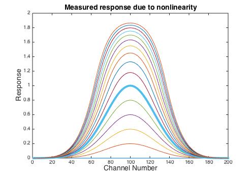
Suppose you have a single component system with a pure component response that is a simple Gaussian peak centered in the spectral range with a maximum value of one when the concentration is also one. Furthermore, suppose that the spectra is linear up to an absorbance of one but rolls off after that. (For x_ideal > 1 I used x_measured = 2-exp(-(x_ideal-1)) but the exact form of the nonlinearity isn’t critical.) The measured spectra for concentrations from 0 to 3 is shown below, with concentration = 1 shown as the thick blue line. It is apparent that the shape changes as the concentration exceeds 1.

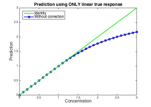
If the concentration is estimated using the ideal (concentration < 1) response, the estimate will fall below the actual value as the concentration passes 1, as shown below. If the spectral residuals were observed it would be apparent that there was a problem, but how to fix it?

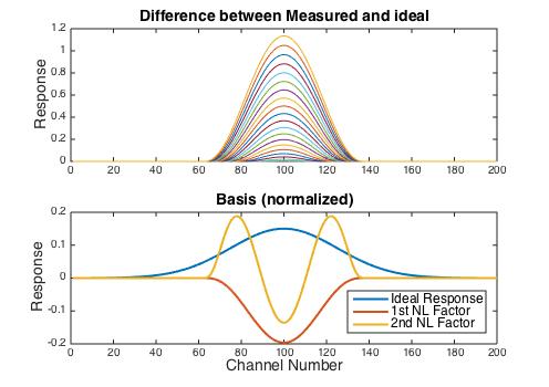
If the ideal response for each concentration is estimated, then the difference between it and the observed response can be calculated, as shown in the top panel in the figure below. Because each difference spectra has a slightly different shape, the rank of this difference matrix is equal to the number of samples exhibiting non-linear behavior, which in this case is 20 (the samples with concentration 1.1 to 3). However, it is easy to get a basis for the nonlinear deviations using the Singular Value Decomposition (SVD). Furthermore, the singular values indicate that 93.7% of the residual sum of squares is captured in the first factor, and 98.6% is captured in the first two. The ideal response along with the first two basis vectors is shown lower panel.

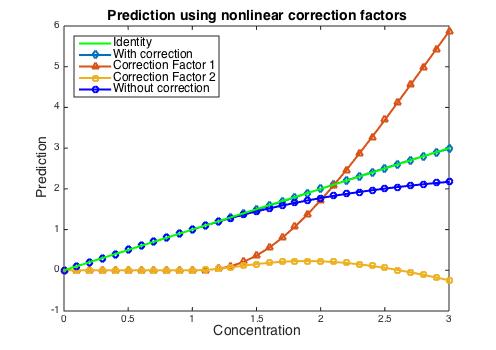
When the CLS model is augmented with the two basis vectors, the prediction improves dramatically. The figure below shows the predicted concentration of the analyte as well as the “concentration” of the two additional basis vector factors. The correction added by the 1st nonlinear factor becomes quite large at high concentrations, whereas the contribution of the 2nd nonlinear factor remains relatively small. The prediction error in the concentration of the analyte is less than 1%.

In a future blog post we’ll explore some other aspects of CLS models.

BMW